12 Zambia (v1)
12.1 Introduction
12.1.1 Background
The richest data on a nation’s population and demographic characteristics usually comes from a national population and housing census. During intercensal years population estimates are produced by projecting census population counts into the future. The UN generates national level population projections for most countries, using well established methodologies (Economic & Social Affairs Population Division 2019) that use national census year population counts, as well as fertility, mortality and international migration rates. National Statistical Offices often produce subnational population projections using similar methods. These subnational areas are usually relatively large in geographic size (e.g. administrative unit level 3) due to the data required for projections (age-sex disaggregated population counts and demographic rates) not being available at lower (finer-scale) administrative unit levels. However, the need for accurate population estimates at a high spatial resolution is echoed throughout governmental, humanitarian and service providing sectors (Tatem 2014). To generate population data at a finer spatial resolution, administrative unit population estimates from projections can be disaggregated across the area within (Bondarenko et al. 2020a). However, the further in time from the original census data population’s are projected, the larger the impact of some key problems relating to data availability and geographical constraints of data on the resulting population projection estimates. These key problems are then propagated into any disaggregated high spatial resolution population estimates that are based on projected population numbers. The key issues include:
- Internal migration between subnational units is often not considered due to lack of data. Similarly, understanding which subnational unit international migrants have moved to and from may be unknown, even when national estimates exist
- Expansion of settlements across subnational administrative unit boundaries, leading to the settlement’s growth incorrectly being projected solely in the settlement’s original unit
- Variation in fertility and mortality rates within administrative units not considered. This may be particularly significant in urban areas where administrative units contain very different settlement types and contexts
- Changes in the boundaries of administrative units and creation of additional administrative units
To address the need for accurate population estimates at a high spatial resolution, particularly when population figures rely on projections over extended time periods, alternative approaches are being developed. One approach, known as the ‘bottom-up’ approach (Wardrop et al. 2018c, Weber et al. 2018b, Leasure et al. 2020g), harnesses population counts for well‐defined, small areas across a country or study region collected more recently than the country’s last census. This approach involves developing a statistical model that best describes the relationship between population densities and variables (geospatial covariates), such as building density or vegetation cover, at survey sample locations. The parameterised statistical model, along with the geospatial covariate values for every location across a country, are then used to predict population estimates at each of these locations.
12.1.2 Zambia Context
The last Zambian population and housing census was conducted in 2010. During 2020 the Zambia Statistics Agency (ZamStats) carried out pre-census cartography fieldwork, in preparation for their upcoming census. To support field work activities, WorldPop worked with ZamStats to produce high-resolution population estimates (at approximately 100m x 100m) based on recently collected survey data. Because these estimates provide local level information about where populations are located, they can be beneficial for planning household level fieldwork and cross-referencing field collected data. One key advantage of our modelling approach is that it provides a measure of uncertainty in the population estimates. This can be useful for planning and carrying out fieldwork by extracting the upper and lower population estimates within a 95% credible interval (CI) and comparing these to the field collected data. For example, if the modelled population estimates for an enumeration area (EA) show a mean value of 1,000, as well as upper and lower 95% CI of 800 and 1,250, respectively, this may indicate that the EA has a suitable population size for field data collection. Additionally, post-fieldwork comparisons between the estimates and field collected population data can be carried out. If fieldwork revealed that 900 people were present in the EA example above, we would conclude that this is within the 95% CI of the population estimates data, however, a population count of 790 or 1,260 from field work would be outside the 95% CI and may indicate that further investigation of that EA is needed. While a discrepancy such as this could be due to inaccuracies in the modelled estimates or the field data, this form of cross-referencing can be helpful for identifying areas missed during field work and/or mismatches between digitised EA boundaries and the area in which field data was collected. In this work we describe the methodology developed for the Zambia population modelling work. We build on previous pioneering work conducting to produce population estimates for Nigeria where Bayesian hierarchical modelling approaches were developed from methods more commonly used in the field of ecology (Leasure et al. 2020g). In contrast to the Nigeria work, here we modelled data from three different surveys that had different survey sampling designs and collected different enumeration related data. The three field enumeration datasets came from the Saving Mothers, Giving Life survey - 2017 (SMGL), the Livestock Census survey - 2018 (LSC) and the pre-‐census Pilot Mapping/Cartography- 2019 (PM). ZamStats anonymised this data prior to access and use for this analysis. A bespoke approach was developed, in both data preparation and modelling, to accommodate for the differences between the surveys and reduce biases in the results. Key elements of this approach include:
- Automating the creation of cluster boundaries from GPS located households to accurately delineate the area surveyed
- Integrating reported households that could not be enumerated into the modelling framework to increase the accuracy of population estimates and uncertainty measures
- Incorporating weighted likelihoods for each sample to accounted for ‘Probability Proportional to Size’ (PPS) sampling strategies that increase the probability of selecting a survey cluster with a larger population count
- Using building footprints data to generate covariates that represent fine scale variability within settlements
12.2 Methods
12.2.1 Data
Survey Data: All survey datasets included counts of population enumerated for each household, with household or building locations (latitude and longitude) recorded using GPS-enabled devices. The key differences between the three survey datasets were: 1. information on households that could not be enumerated (missing households); 2. spatial coverage; and, 3. site location selection (survey sample design). Missing households data was present for LSC and PM, but absent for SMGL. LSC consisted of sample locations across the whole country, while PM consisted of full enumeration across two districts and SMGL consisted of almost full coverage across four areas, each consisting of multiple districts. No site selection process was used for PM and SMGL as they aimed to survey everywhere within their target regions, however, LSC employed a probability proportional to size (PPS) sampling design. For the sampling approach of LSC, the country was first stratified by districts and then enumeration areas (EAs) were selected by weighting EAs within each district by their number of households according to the 2010 census household listing data.
Population densities at each survey location are required for the statistical model, and therefore to accurately calculate population density, we need to know both the exact area that was covered in the survey fieldwork and the population count for the survey cluster/enumeration area. Digitised survey cluster boundaries were unavailable for these three surveys. However, GPS locations of households (point locations) were provided which allowed us to demarcate the area covered during field data collection.
The following three sections describe the individual surveys and how their data were prepared for the modelling.
Pilot mapping/cartography : This data identified the location of all residential buildings as well as non-residential areas across the two districts, Lusaka and Chongwe. Data point locations were cross-checked and verified using multiple geo-location variables included in the data. Because the point data covered two districts, it was necessary to sub-divide the data into smaller units; the study area was objectively split up into 1km x 1km blocks. The blocks not on the edge of the study area were classed as ‘clusters’ with the 1km x 1km block demarcating the cluster boundary. The 1km x 1km size of the blocks was used because: a) smaller sizes would have led to a larger number of points being potentially assigned to the wrong clusters due to GPS error, and b) larger sizes would have led to many clusters having very large population counts. The aim of the 1km x 1km size was to obtain clusters comparable to those in the two other survey datasets whilst maintaining objectivity in the approach. Blocks on the edge of the study area included areas not covered by the survey, and therefore bespoke cluster boundaries were created around the GPS points inside these ‘edge’ blocks. These cluster boundaries were generated using the R function ahull (Pateiro-López & Rodríguez-Casal 2010, Dauby 2019). We required a minimum of 15 points to create a cluster boundary because situations with less than 15 points could result in high uncertainty in the exact location of the boundaries, leading to an incorrect demarcation of the settled area for which data was collected. Clusters were not created for ‘edge’ blocks with less than 15 GPS points and therefore these areas were excluded. This approach of creating cluster areas from the larger study region was aimed to be objective, however, we did not investigate potential impact of this demarcation approach on the results. Future work needed to understand how sensitive the statistical model might be to different cluster demarcations is outlined in the discussion section of this report. This dataset included information about households (in residential buildings) where enumeration was not possible, e.g. due to non-response (no one answering the door). A small number of non-responders in household surveys is common and, in this survey, well documented. This information is incredibly useful for population modelling because it allows for uncertainty in the observed population counts to be modelled. In order to calculate accurate proportions of missing household counts per cluster we first identified the data points that were residential. We classified points as residential if their structure type was categorised as a ‘Residential building’ or if the residential building variable was non-NA. This allowed households classified as ‘residential’ or ‘multi-purpose’ to be included as our aim was to identify all the buildings where people lived. Second, we identified erroneous household sizes and replaced them with NAs. There were three obvious data entry mistakes (population counts per building of 1000000018, 999999 and 40004) and three more where values were between 200 and 1,000. Visual inspection of data points and building footprints surrounding these three potentially erroneous household sizes verified that they were almost certainly errors, as their building footprints looked similar to nearby footprints with corresponding household counts of between 1 and 15 and were clearly not counts for several buildings. All six household counts above 200 people were replaced with NA household sizes and treated as missing household counts. The next largest household size was 139 for a block of flats (enumerated as one household). All household sizes below 140 were therefore assumed to be correct.
Livestock census survey: – This dataset included a nationally representative sample of survey clusters. As this survey used probability proportional to size (PPS) sampling, we needed the survey weights for each cluster. There were four clusters without survey weights data and these were therefore excluded. Although cluster boundaries were unavailable, cluster IDs were given for the GPS located households (point locations) making demarcation of the cluster areas possible. Any GPS locations outside of the country were replaced with NAs, i.e. unknown location, and any clusters that did not have GPS locations for at least 95% of listed households were excluded, as accurate demarcation of clusters was only possible where a high proportion of the household locations was known. While survey data collected with GPS coordinates can lead to improved knowledge of the exact area covered during fieldwork compared to using standardised digitised boundaries, it can also lead to discrepancies in some cases. These include a) GPS points from different clusters having significant overlap, and b) grouping of GPS points in a very small non-residential area far away from the rest of the cluster’s points. The latter most likely occurs if data was ‘logged’ by the GPS devise after surveyors returned to their ‘base’. Because of associated issues in determining the exact area covered during fieldwork where discrepancies in GPS locations exist, we exclude clusters with significantly overlapping GPS locations and those with more than one grouping of at least 5 GPS points with obvious settled area in between groupings. Where clusters had fewer than 5 GPS locations clearly not at their cluster site, these GPS locations were replaced with NAs and the 95% threshold for valid GPS points per cluster was applied. For clusters meeting the 95% threshold of valid GPS points, cluster boundaries were generated using the R function ahull, as was done for the ‘edge’ areas of the pilot mapping dataset (described above). All clusters post- data cleaning had 15 or more points, and therefore no further clusters were excluded before creating cluster boundaries.
Saving Mothers, Giving Life survey: – This dataset contained GPS located households for four regions. Like the livestock census data, GPS points were linked to cluster IDs and we therefore followed the same procedures for demarcation of cluster boundaries. These were: 1) replacing any GPS locations outside of the country with NAs, 2) excluding clusters that did not have GPS points for at least 95% of the total number of households recorded, 3) excluding clusters with significant overlap in GPS locations (which was very common in urban areas of the SMGL data, however, only 11% of the SMGL clusters were urban), 4) excluding any clusters with less than 15 points, and 5) creating cluster boundaries using the R function ahull.
The cluster level survey data from the three surveys were then combined to create the model input dataset. The proportions of missing households per cluster were calculated for the livestock census survey and pilot mapping datasets. The SMGL data did not include information about missing households. We address this unknown factor in our modelling approach and make use of the existing missing households data from the livestock census survey and pilot mapping to parameterise the missing households sub-model section of our statistical model. This allows for the uncertainty in cluster population counts for the SMGL data to be accurately accounted for.
To reduce the uncertainty in our results, clusters from the livestock census survey and pilot mapping with more than 20% of missing household size data were excluded from the input data used to fit the regression model. There were no spatial biases in these excluded clusters. Where survey clusters from different surveys overlapped, the most recently collected survey cluster was kept to avoid pseudo-replication (Hurlbert 1984). Additionally, one cluster was dropped (pilot mapping) because it contained just one person. The final dataset included 2,605 clusters. Figure 12.1 shows the spatial distribution of the clusters and Figure 12.2 shows the number of clusters by survey and settlement type.
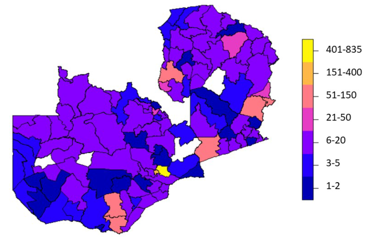
Figure 12.1: Number of survey clusters per district included in the population modelling. Four districts out of 116 districts of Zambia had no clusters (white). The total number of clusters was 2,605. Note, these are not official government boundaries. The production of this boundaries dataset was facilitated by GRID3 in collaboration with the Government of Zambia (Ministry of Lands, Ministry of Local Government, Zambia Statistics Agency, Electoral Commission of Zambia).
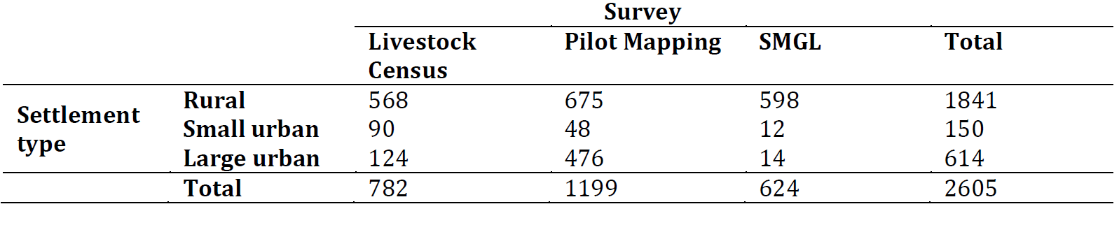
Figure 12.2: Final number of survey clusters by survey and settlement type used for the regression model.
Because the Livestock census survey was conducted using probability proportional to size (PPS) sampling, we needed to account for the fact that the dataset is biased towards clusters with larger population sizes. The survey weights (the relative measure of how representative a cluster is of the wider population) were included in the survey data. Survey weights for pilot cartography and SMGL were assumed to be equal across all their clusters (i.e. random sampling) and the single survey weight value assigned to them was the mean survey weight from the livestock census survey. This results in the model putting equal weight on the pilot cartography and SMGL clusters, whilst the weight varies for the livestock census clusters where, generally, clusters with lower population sizes have a higher survey weight to account for the bias in the sample design where higher population clusters were more likely to be selected and surveyed. We normalised (scaled to sum to one) the survey weights to produce model weights which were then used in the statistical model to reduce biases due to survey sample design. There is inherently additional bias due to the SMGL and pilot mapping data being spatially targeted. While we did not explicitly account for this bias, the spatial hierarchical nature of our statistical model leads to inferences within any given district and settlement type to rely more on the data from the same district and settlement type. Because of this we expect district-settlement type pairs that were well represented in the data not to be heavily influenced by any spatial biases of the overall input dataset. However, those district-settlement type pairs not well represented may be impacted by spatial biases in the data especially if they were in the same province as the concentrated clusters.
12.2.1.1 Geospatial Covariates
We used province and district boundaries in our statistical model. The production of the boundaries dataset used was facilitated by GRID3 in collaboration with the Government of Zambia (Ministry of Lands, Ministry of Local Government, Zambia Statistics Agency, Electoral Commission of Zambia) and are not official government boundaries. For this work we rasterised the boundaries using the WorldPop WGS84 projected raster master grid for Zambia (WorldPop 2018b).
For the statistical modelling we determined the relationship between population density and predictive variables. Our measure of population density was population per total building area, where building area included both residential and non-residential buildings. All building footprint related geospatial layers were created using building footprints provided by the Digitize Africa project of Ecopia.AI and Maxar Technologies (Ecopia.AI & Maxar Technologies 2020b). The building footprints data includes extremely large structures such as stadiums, but also detects solar farms as large ‘structures’ too. Because it is unlikely that people will be living in these exceptionally large structures, we did not want the final population dataset to include people in grid cells that contain these large structures only, and so we applied a building area threshold of \(750m^2\) to filter out very large buildings. Note that it is unlikely that this led to the exclusion of any flats or dormitories. After filtering out very large buildings we generated gridded geospatial (raster) layers for metrics of the remaining buildings. To do this we first converted building footprint polygons into building centroid points in UTM projection using the st_centroid function in the sf R package (Pebesma 2018b). The centroid points were then re-projected to WGS84 using the st_transform function so that their corresponding cell IDs in the WGS84 projected master grid raster could be identified. Building centroid cell IDs were obtained using the cellFromXY function in the raster R package (Hijmans et al. 2015b). Building counts per grid cell were calculated by simply summing the number of centroids for each cell ID. Building density per grid cell was calculated by dividing the building count in a cell by the area of the cell. Grid cell area was calculated using the area function in the raster R package. To calculate cluster-level mean building density we took the mean of density values across all settled pixels within a cluster’s boundary. The three building area-related layers were all derived using the “Shape_Area” attribute contained in the .gdb building footprints dataset, by applying sum (total area), mean and coefficient of variation (standard deviation divided by mean), for the focal area (either grid cell or cluster areas). We categorised each grid cell with at least one building footprint centroid as either rural, small urban or large urban, based on the size of the settlement they belong to. Grid cells in clusters smaller than 500 cells were classed as rural. Grid cells within clusters of 500 to 1,500 contiguous grid cells were classed as small urban. Grid cells within clusters of more than 1,500 contiguous grid cells were classed as large urban. The clump function in the raster R package was used to identify clusters of contiguous cells; grid cells were classified as being in the same cluster if they were directly adjacent to any of the eight neighbouring grid cells, including diagonally adjacent (Queen contiguity). To assess potential impact of the age of imagery used to extract the building footprints, we summarised imagery ages for all building footprints included in the survey clusters (used in the modelling) and across the whole country (used in the predictions).
12.2.2 Statistical Modelling
The goal of this work was to build and parameterise a statistical model that could then be used to predict population counts across every 100m x 100m grid cell of Zambia. We used a Bayesian statistical approach as this allowed us the flexibility to build a model that could account for known uncertainties in the observed data, therefore allowing us to produce results with realistic uncertainty in the population estimates. The model we used includes a core regression model (Equation (8.4)) that accounts for biases in the observed data due to population weighted sampling design (Equation (8.3)) and (Equation (8.5)) and an observation error sub-model that accounts for uncertainty in the observed data due to missing households (Equation (8.1)). The core regression model describes the relationship between population density (\(D_i\)) and the three predictor variables (covariates):
- log mean building footprint area (\(X_{1, i}\)),
- log mean building footprint density (\(X_{2, i}\)), and
- coefficient of variation in building area (\(X_{3, i}\)). The regression has a hierarchical random intercept where districts are nested within provinces and provinces are nested within settlement type. This structure allowed us to account for similarities between observed data within the same district, province and settlement type that cannot be explained by the covariates. Such similarities may result from local level social and cultural trends that are difficult to measure. In the final statistical model used for the predictions, i.e. the model that predicted the observed data well, two of the covariates (\(X_{2, i}\) and \(X_{3, i}\)) had coefficients varying by settlement type (\(\delta_{s}\) and \(\gamma_{s}\)). To account for biases due to survey sampling designs we used model weights for each cluster (described in the data preparation section). If the model weight was relatively low, that cluster’s population density value would contribute less to the fitting of the model compared to clusters with higher model weights. This is implemented in (Equation (8.3)) and ((8.5)) of the model where the precision \(\tau_{i}\) of the population density (\(D_i\)) estimated for a cluster is adjusted by the model weight (\(w_i\)). Where survey clusters have households that were not enumerated, we did not know the exact number of people in those clusters. The larger the number of missing households in a cluster, the larger the range of possible population counts for that cluster. Therefore, clusters with a large number of missing households will have a larger uncertainty in their population counts. We incorporated this uncertainty in the statistical model via an observation error sub-model shown in (Equation (8.1)). For the livestock census and pilot cartography clusters the number of missing households were known and the parameter values of the binomial were calculated directly from the cluster level data. For the SMGL survey we did not know how many missing households there were in each cluster and we therefore needed to determine the parameter values of the binomial for the SMGL clusters using information from the other surveys. First, we calculated the proportion of non-missing households (i.e. proportion of total households that were enumerated) for every cluster surveyed in the livestock census and pilot cartography (\(n = 3,489\)). This provided information about the probabilities associated with different proportions of enumerated households per cluster across two full surveys (Fig. 12.3).
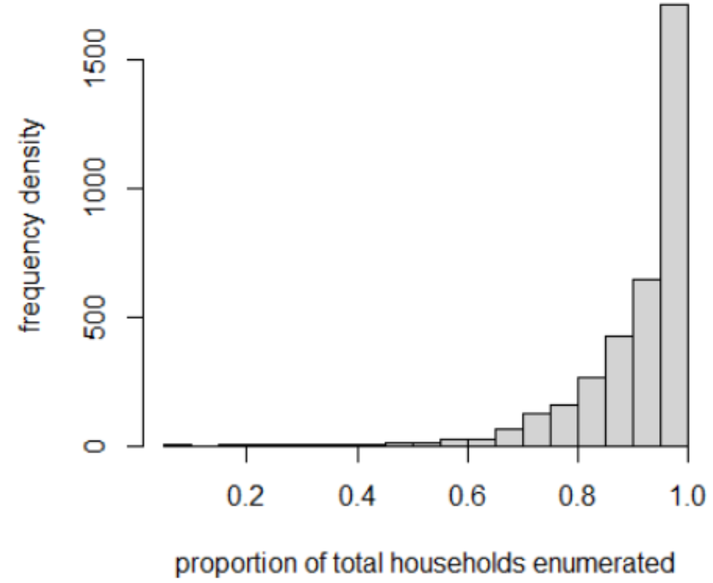
Figure 12.3: Frequency distribution of the proportion of total households enumerated in a survey cluster across two surveys (pilot mapping and livestock census survey); n=3,489.
We then used this probability distribution to fit the \(prop_i\) parameter in (Equation (8.1)) for SMGL clusters. In each survey cluster \(i\), the field enumerators counted \(P_i\) people, but there were also potentially some households that were unobserved. We included this process as an observation model:
\[\begin{equation} P_i \sim \text{Binomial}(N_i, \theta_{i}) \\ \theta_i = 1 - \frac{(mhhs_i (\frac{nhh_i}{prop_i} - nhh_i))}{N_i}\tag{8.1} \end{equation}\]
where \(N_i\) is the total number of people in the cluster (observed and unobserved) and \(\theta_i\) is the probability that a person who resided in the cluster was counted during the enumeration. The primary purpose of this portion of the model is to estimate the total number of people \(N_i\) in the cluster. We calculated the observation probability \(\theta_i\) deterministically based on the mean household size \(mhhs_i\), number of households enumerated \(nhh_i\), and the proportion of the total households that were enumerated \(prop_i\).
We also used the observation model to estimate the parameter \(prop_i\) using the observed data from two surveys (livestock census and pilot cartography) to infer these values for the survey where they were not available (SMGL). For this purpose, we modelled \(prop_i\) as a stochastic parameter rather than treating it solely as observed data:
\[\begin{equation} prop_i \sim \text{Beta}(5, \pi)\tag{8.3} \end{equation}\]
where \(\pi\) is a shape parameter estimated to fit this beta distribution to the observed data.
The next portion of the model was designed to estimate the population density \(D_i\) for each cluster \(i\) based on the estimate of total population \(N_i\) (above) and the observed total building area \(A_i\):
\[\begin{equation} N_i \sim \text{Poisson}(D_iA_i)\tag{8.4} \end{equation}\]
\[\begin{equation} D_i \sim \text{LogNormal}(\mu_i, \tau_i)\tag{8.5} \end{equation}\]
where \(\mu_i\) is the expected population density (i.e. the mean of the lognormal distribution) for cluster \(i\) and \(\tau_i\) is the precision of that expectation. Note that precision is the inverse of variance (\(\tau_i\) = \(\frac{1} {\sigma^2}\)) and this term provides a measure of uncertainty (i.e. residual variance).
We modelled the expected population density \(\mu_i\) as a linear function of the set of covariates \(X_i\):
\[\begin{equation} \mu_i = \alpha_{s,p,d} + \beta X_{1,i} + \delta_s X_{2,i} + \gamma_s X_{3,i} \tag{8.6} \end{equation}\]
We used a hierarchical random intercept to account for correlations among clusters in the same settlement type \(s\), province \(p\), and division \(d\). We also used random slopes for two covariates (\(X_2\) and \(X_3\)) to estimate the effects of these covariates for each settlement type \(s\). Samples that were collected for the livestock census survey used a PPS sampling design rather than random sampling. PPS sampling design may result in a sample that contains more data from areas with high population density, which would bias our estimates of population density \(D_i\) if not accounted for. We used a weighted-precision approach (similar to weighted-likelihood or inverse-variance weighting) to account for this:
\[\begin{equation} \tau_i = w_{i}/\sigma^2_{s,p,d} \tag{8.7} \end{equation}\]
where \(w_i\) are the model weights (described above). These model weights are the inverse of the probability that a cluster was selected for the survey. This weighted-precision model decreases the influence of clusters from high population density areas that were over-represented in the sample compared to lower population density areas that were under-represented in the sample. This provides an unbiased estimator of population density from non-random weighted survey data.
The model was fit using JAGS v4.3.0 (Plummer 2003b) where 3 chains were run, each with burn-in and adapt phases of 10,000 and 1,000 iterations, respectively. A total of 35,000 iterations per chain were run in the post-burnin and -adapt phases. To eliminate autocorrelation among a parameter’s estimates within a chain, iterations were thinned so that every 3rd iteration was kept. We checked for model convergence using the \(gelman.diag\) function in the coda R package which allows the potential scale reduction factor (psrf) values to be calculated (Plummer et al. 2006). The psrf is a measure of the variance between chains compared to the variance within chains. When these variances are similar, the chains have reached their target distribution and therefore psrf scores less than 1.1 indicate chain convergence. In instances where the psrf score was above 1.1 we continued running the model until model convergence was achieved.
To check that the model is not overfitting to the data, we performed 10-fold cross validation. This involved re-running the model 10 times with a different 10% of the input data held out in each run. As with the original model, each cross validation model was run until either model convergence was achieved or for 35,000 iterations without convergence. Across all cross validation models, nine (out of 2605) posterior \(N_i\) (population counts) and/or \(D_i\) (population densities) did not fully converge, although all had a psrf score of <1.3. Running the relevant cross validation models for longer may produce slightly more accurate cross validation results, however, we confirmed that none of the nine predictions had a corresponding observed value outside of the 95% CI and so we believe that this would make very little difference to the results.
12.2.3 Predictions and Final Dataset
For every ~100m x 100m grid cell across Zambia we calculated the probability distribution of population counts (i.e. posterior predictions) using a grid cell’s covariate values and the parameterised model above. Note that the missing households sub-model aimed to allow for accurate parameterisation of the regression model, and is not needed for the predictions where we were estimating \(N_i\) not \(P_i\). The grid cell level posterior distributions are available in the SQL database (‘ZMB_population_v1_0_sql.sql’) of the publicly available dataset WOPR. The mean of the posterior predictions for grid cell level population estimates can be found in the raster file (ZMB_population_v1_0_gridded.tif) in WOPR. To enable users to quickly identify areas of comparatively high and low uncertainty in the mean population estimates, we generated a complementary uncertainty raster file (ZMB_population_v1_0_uncertainty.tif) in WOPR. The uncertainty values here are the difference between the upper and lower 95% CI of the probability distribution divided by the mean of the probability distribution: \((upper - lower)/mean\). This layer offers one measure of uncertainty and alternative measures can be calculated using the SQL database. Uncertainty estimates cannot be summed across grid cells to produce an uncertainty measure for a multi-cell area. Uncertainty for larger areas should be calculated by summing the grid cell level probability distributions to generate a new probability distribution for that area, from which the correct uncertainty measure can be calculated. This process is automated by the woprVision web application WOPR Vision and the wopr R package (Leasure et al. 2021a). To accompany district and province mean population estimates, we have pre-calculated the upper and lower 95% CI, and these are available in the ZMB_population_v1_0_admin.zip shapefiles WOPR. We also produced population estimates for individual age-sex groups by multiplying the gridded mean population estimates (ZMB_population_v1_0_gridded.tif) by regional level age-sex proportions. These proportions are accessible via this portal AGE SEX. All data processing and analysis was carried out using R (v.3.6.0) (R Core Team 2013) with the exception of the rasterization of the district and province boundaries which was carried out in ArcGIS Pro.
12.3 Results
12.3.1 Assessment of Building Footprints Data
The building footprints data largely represents a recent distribution of buildings. Across the whole country, 93% of the building footprints were extracted from imagery between 2017 and 2019, and across the clusters used to fit the statistical model, this was 96%. In Figure 12.4, we present summaries of the distribution of building footprints across imagery years, and Figure 12.5 shows a histogram of building footprints imagery dates by month for all building footprints used in for the grid cell level population predictions. From these assessments we do not believe there is any significant mismatch in the building footprints and the dates the survey data were collected. For the 7% of the country where building footprints represent dates earlier than 2017, we advise that the gridded population estimates be used with caution. The modal year of the Zambia building footprints for each grid cell are available in Dooley et al. (2020).
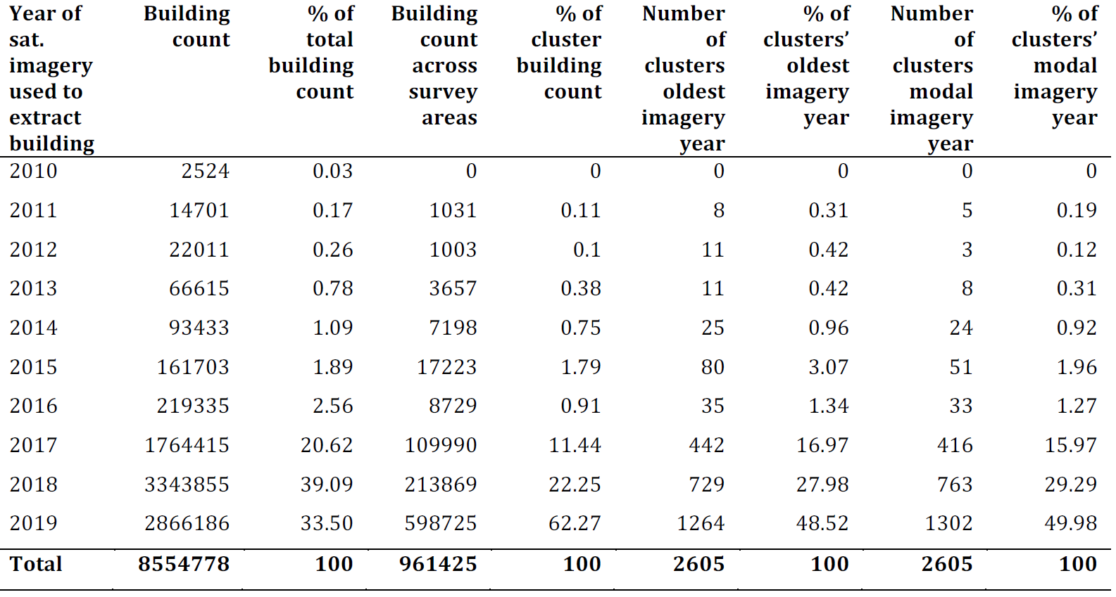
Figure 12.4: Distributions of building level imagery years for buildings used in the grid cell level predictions (columns 2 and 3), and cluster level model fitting (columns 4 to 9).
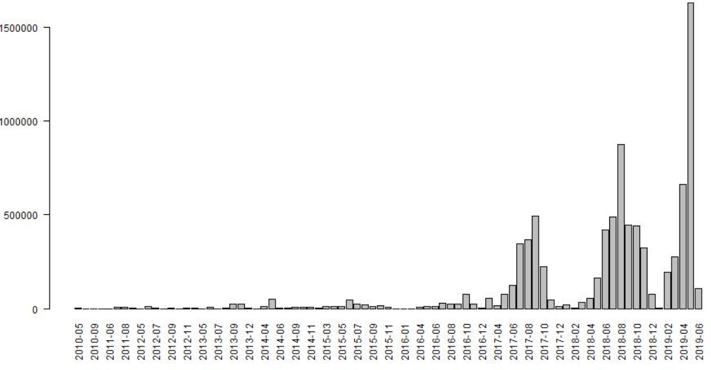
Figure 12.5: Histogram of building footprints imagery date for all building footprints used for the grid cell level population predictions.
12.3.2 Model Fit
For assessing model fit we compare observed and predicted \(N_i\) (true population count) and \(D_i\) (population densities). As we did not have the observed number of missing households for the SMGL survey, we did not have an observed \(N_i\) for SMGL clusters (just observed \(P_i\) values). We could have used the modelled mean estimate of missing households to calculate \(N_i\) for SMGL clusters but this would have likely led to overstating the model fit. To present a more conservative assessment of model fit we examined observed and predicted \(N_i\) and \(D_i\) for PM and LSC clusters only. Due to unknown population counts for any missing households, we calculated observed \(N_i\) by assuming missing households have a population count equal to their cluster’s mean household size. Given that we filtered clusters such that they must include at least 80% of total households enumerated, we believe that this is a reasonable value for observed \(N_i\) to assess model fit. Observed vs predicted \(N_i\) and \(D_i\) are shown in Figure 12.6 for both in-sample and out-of-sample (cross-validation) results.
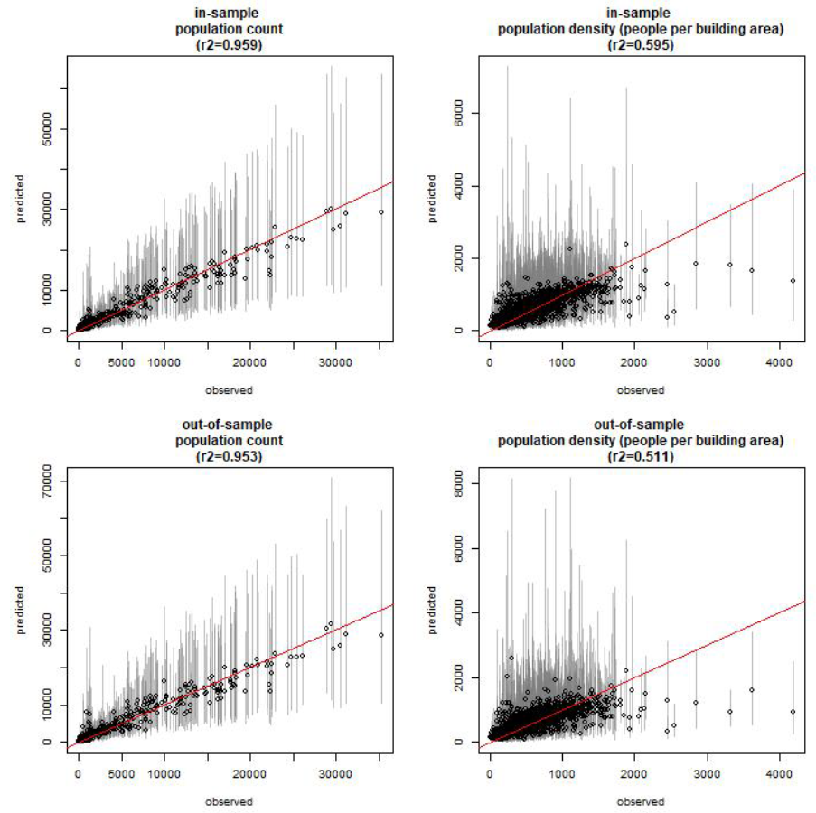
Figure 12.6: In-sample and out-of-sample observed vs predicted population counts \(N_i\) and population densities \(D_i\) (people per total building area); n=1981. Circles represent the cluster mean prediction and lines show their corresponding 95% credible intervals.
The corresponding model statistics are presented in Figure 12.7. The model statistic results show that model performance is maintained when 10% of the input data is held out, indicating that the model is not overfitting to the data. We find a very high correlation between observed and predicted population counts (\(R^2\) = 0.959 for in-sample \(N_i\)) and lower correlation between observed and predicted population densities (\(R^2\) = 0.595 for in-sample \(D_i\)). This suggests that the population densities responsible for lowered correlation between observed and predicted values, correspond to clusters with small total building area as they have little consequence on the overall correlation between observed and predicted population count. These results are not surprising given that the data included clusters with very small population sizes, across which the variation in number of buildings per cluster will result in higher variation in population density, compared to clusters with relatively large population counts. In other words, over a threshold number of buildings, population densities typical of the area can be calculated more accurately. For future testing of the model, we could assess model fit when clusters below a threshold population size are excluded from the input data.
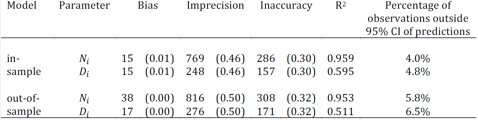
Figure 12.7: Results of model statistics for in-sample and out-of-sample (cross validation). Statistics shown are bias (mean of residuals), imprecision (standard deviation of residuals), inaccuracy (mean of absolute residuals) and R-squared (\(R^2\), correlation between absolute observed and predicted values). \(N_i\) is the true population count and \(D_i\) is population density (people per building area). Numbers given for bias, imprecision and inaccuracy are people with the standardised values (i.e. divided by predicted \(N_i\) or \(D_i\)) in parentheses. By random chance we expect the percentage of observations outside the predicted 95% credible intervals (CI) to be ~5%.
In addition to the correlations between observed vs prediction values, as described above, we checked for spatial autocorrelation in the standardised residuals ((mean prediction values - observed)/observed). The standardised residuals give a measure of variance in the data unexplained by the model and therefore commonalities among clusters with similar residual values indicates that the model could be improved if those commonalities were accounted for. There is little evidence for spatial autocorrelation in the standardised residuals, as shown in Figure 12.8, which suggests that the model accounts for spatial variation well.
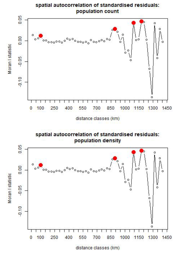
Figure 12.8: Spatial autocorrelation in standardised residuals (variance unexplained by the statistical model) for population counts (top) and densities (bottom). Red dots indicate the distances at which there is significant spatial autocorrelations. These occur between clusters that are ~100 km, ~ 900 km, ~1,100 km and ~1,175 km apart.
To understand whether the model is capturing the uncertainty in the data well, we draw our attention the 95% CIs. By random chance we expect the percentage of observations outside the predicted 95% credible intervals (CI) to be ~5% or lower. Figure 12.7 shows that <5% and <7% of observations were outside the predicted 95% CI for in-sample and out-of-sample results, respectively. While this demonstrates that the model is capturing uncertainty well, we looked for commonalities among the instances where observations were outside the predicted 95% CIs to investigate whether we can make improvements to the model. Generally we found little evidence for biases across the full set of clusters with observations outside the 95% CIs, however, we did identify three common features among small groups of clusters where 95% CI predictions consistently miss the observed value.
The first is overprediction in six clusters that are located in the industrial area of central Lusaka. The second and third occur in some rural pilot mapping clusters in north Chongwe. For one set there is underprediction and for another there is overprediction. For the set where observed counts (and densities) are higher than the 95% CIs predictions, i.e. model underprediction, the people per household are in-line with the wider data set (see Fig. 12.9), suggesting that these clusters contain a relatively small number of building footprints compared to other clusters. The date of the imagery used to extract building footprints in this area is just a few months after the survey data collection so it is unlikely that there is a mismatch in the building footprints and the surveyed buildings. Further assessment of how these clusters differ to other rural clusters may be required here.
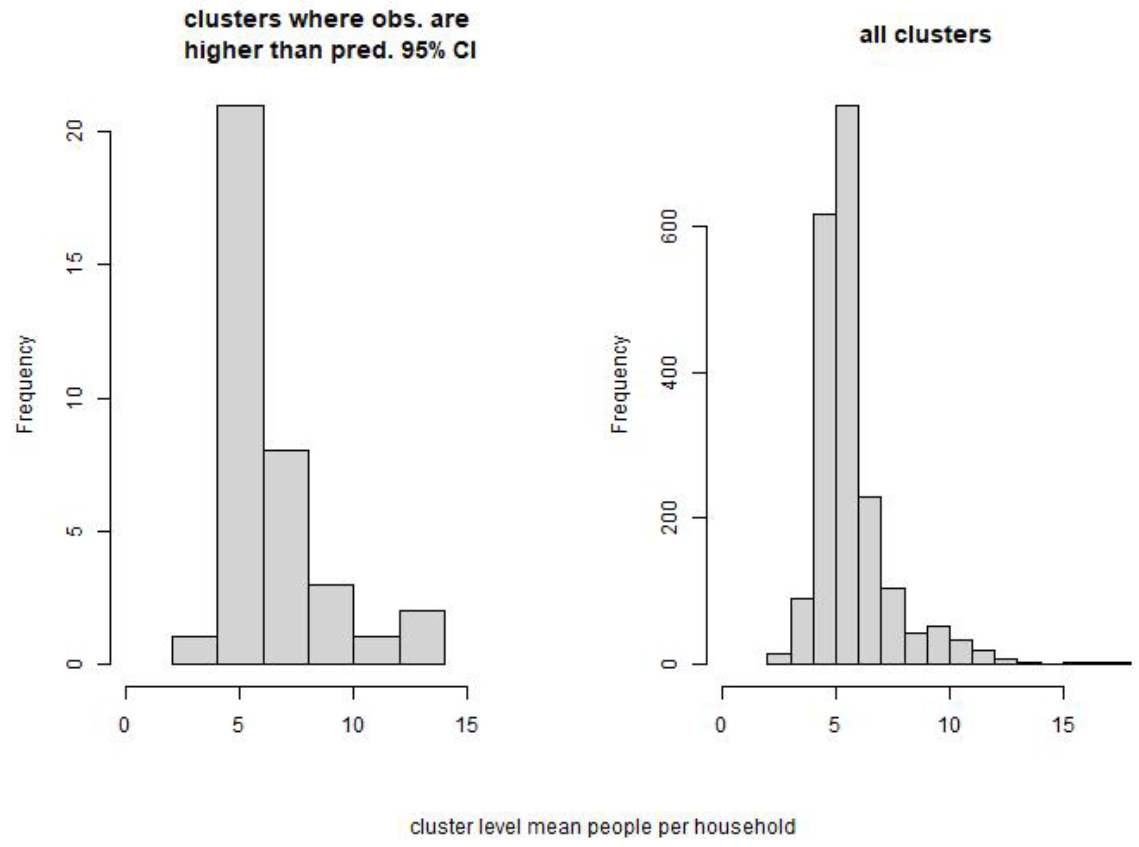
Figure 12.9: Comparison of people per households for clusters where the observed population count is larger than the predicted 95% CIs (left) and all clusters (right).
For the set where observed counts (and densities) are lower than the 95% CIs predictions, i.e. model overprediction, it is likely that the clusters contain areas that were not surveyed as there are sections of the clusters that do not have GPS locations and, again, here there is no mismatch in the dates of the survey and the building footprints. To improve our data analysis we could delineate cluster boundaries in the rural areas based on the GPS locations instead of the block approach, however, given the building footprints we believe that predictions in these few clusters are realistic and that the ‘overprediction’ is in fact due to errors in population density brought about by the clusters including unsurveyed buildings. For data points (locations) where the model describes the data well there will be low uncertainty in the mean prediction. Conversely, we find high uncertainty (wide 95% CI) where the model explains less of the observed variance in population densities. Figure 12.10 shows two example areas where there is relatively high uncertainty in the population estimates. In the Solwezi example, we note that one of the five survey clusters in the south-west of the city has a much lower observed population density than the other four clusters. All five cluster areas are residential with relatively high building density (compared to all other clusters) and have similar covariate values to one another. The low density of one of these cluster is therefore surprising. Further investigation of the low density cluster reveals that a section inside the cluster boundary that contains buildings (according to the building footprints) have no GPS located households. This results in the population density being lower than expected given the other four similar survey clusters in close proximity. There may be a number of possible reasons for this: a) the area could have been undergoing development at the time of the survey (early 2018) and the new buildings are present in the building footprints (imagery year for this area is 2019); b) the fieldwork may not have been complete; or, c) there may have been an error in collating/transferring the data. We make similar observations for the Chirundu example.
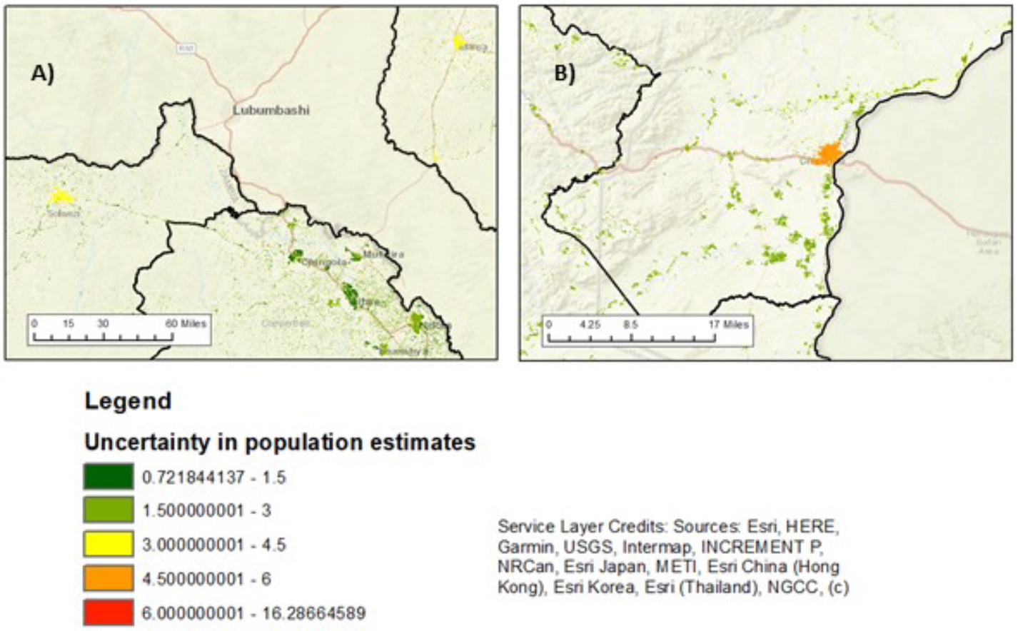
Figure 12.10: Areas of high uncertainty in the modelled population estimates. A) shows relatively high uncertainty for Solwezi (North-Western) and Mansa (Luapula), compared to other urban centres in Copperbelt. B) shows high uncertainty levels in Chirundu’s population estimates.
12.3.3 Summary of Population Estimates
The national modelled mean population estimate for Zambia is 21,672,678 (lower and upper 95% CI: 20,929,048 and 22,491,208). Population estimates per province is provided below in Figure 12.11.
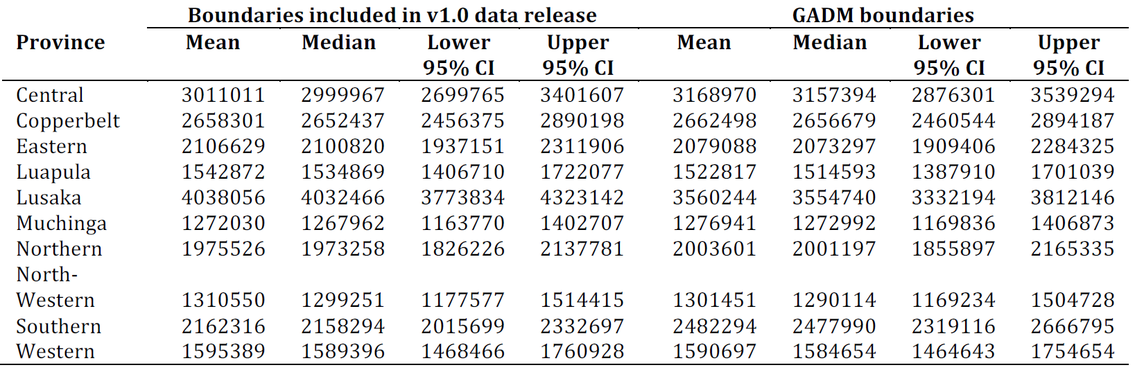
Figure 12.11: Modelled population estimates per province for two different boundaries datasets. The production of the boundaries dataset included in modelled population data set v1.0 was facilitated by GRID3 in collaboration with the Government of Zambia (Ministry of Lands, Ministry of Local Government, Zambia Statistics Agency). Note that both boundary datasets are not official government boundaries.
12.4 Discussion
All model assessments suggest that the statistical model that we developed performed well and was appropriate for predicting population estimates across Zambia. There was little evidence of mismatch in the dates of survey data collection and building footprints, and we therefore believe that the gridded population estimates represent a realistic distribution of the Zambian population around 2018/2019. We encourage users of the modelled population estimates to consult the uncertainty measures via the uncertainty raster and/or the woprVision WOPR Vision web application (select “ZMB v1.0”) or the wopr R package (Leasure et al. 2021a). We note that there is particularly high uncertainty in the urban centres of Solwezi and Chirundu, and highlight that caution should be taken when using the estimates for the industrial area in central Lusaka and the small areas where the building footprints data correspond to 2016 or earlier.
In the short term, the estimates could potentially be improved by re-fitting the model parameters using input data that excludes clusters with very small population counts and carrying out a sensitivity analysis for the survey weights assigned to the pilot mapping and SMGL clusters to assess any impact these might have. In the longer term, we suggest several areas for future research using these survey data:
Developing methods to create clusters from surveys that cover large areas like the pilot mapping. We took an objective approach of splitting up the area into blocks so that the impact of GPS error was minimal. Future work could include developing cluster boundaries for target population counts that optimise uncertainties in cluster population and building counts.
Exploring the integration of uncertainties in cluster building counts due to cluster boundary locations based on estimated number of buildings within certain distances of the boundaries.
Mapping areas that are predominantly non-residential and, if there are enough survey data covering these areas, incorporating this class of settlement as a fourth settlement type in the statistical model. Methods for classifying settlement types, such as those described in Jochem et al (Jochem et al. 2021b), could potentially be use for identify non-residential areas in Zambia.
Additionally, future work should be done to understand and improve the reporting of missing households so that refinements to the observation error sub-model can be carried out.
Note: The gridded population estimates for the Zambia are available from the WorldPop Open Population Repository WOPR, and they can be visualized using the WOPR Vision web application (select “ZMB v1.0”)
Contribution
The modelling work was led by Claire Dooley with support from Douglas Leasure. Geospatial data processing was carried out by Heather R. Chamberlain and Oliver Pannell. Oversight of the work was provided by by Attila N. Lazar and Andy Tatem