15 Geostatistical Use Cases
Efficient Bayesian Hierarchical Population Estimation Modelling using INLA-SPDE: Integrating Multiple Data Sources and Spatial Autocorrelation
15.1 Introduction
Small area population count data support decision-making across all areas of governance. Estimating population numbers affected by disasters, delivering health interventions, planning for elections and allocating resources equitably all require reliable estimates of population distributions at small area scales (UNFPA 2020b). Such data are typically collected through a national population and housing census, but these can become quickly outdated in settings with substantial population movements and heterogeneous patterns of fertility and mortality that are hard to predict (Tatem 2022). In addition, in some areas of certain countries, it is sometimes not possible to directly collect such population data due to conflicts or other security challenges. To fill these data gaps, geospatial methods have recently been developed that leverage advances in satellite imagery, computer vision, geospatial computation and spatial statistics to produce small area population estimates across national extents (e.g Leasure et al. 2020h, Boo et al. 2022b, Darin et al. 2022b). ‘Bottom-up’ population models leverage the statistical relationships between population density measures in incomplete enumerations of an area of interest and a set of geospatial datasets capturing features known to correlate with how humans distribute themselves on the landscape. The enumeration data can come from purposely designed microcensus surveys (e.g Leasure et al. 2020h, Boo et al. 2022b), incomplete census enumeration (e.g Darin et al. 2022b), or listings from household surveys (e.g Dooley et al. 2020c). Predictions of numbers of residents for 100m by 100m grid cells are then typically made, and the use of Bayesian statistical inference methods for the estimation of the population model parameters means that estimates of uncertainties can be provided (Wardrop et al. 2018d).
Potential sources of estimation and prediction biases exist in the production of bottom-up model-based estimates. For example, the differences between the spatial scales of the data observation units or statistical model estimation units and that of the high-resolution population prediction grid cells are a potential source of prediction and aggregation biases that have not been fully addressed and its effects on the accuracy of population predictions are largely unknown (e.g Paige et al. 2022). Moreover, the need to explicitly account for potential sources of errors in spatial statistical models that often require the aggregation of point estimates to obtain areal level estimates has been the major focus of recent studies within the spatial statistical domain (Lee et al. 2022, Paige et al. 2022). Indeed, spatial statistical models which account for unobserved effects of inherent spatial autocorrelations within the observed spatially referenced data have been shown to minimize estimation biases, produce more accurate predictions and provide a clearer picture of the spatial patterns of the response variable of interest, whether in infectious disease studies (Wakefield 2007, Lee 2011, Diggle & Giorgi 2016b, Giorgi et al. 2018), human mobility studies (Carella et al. 2022), or fish population and distribution studies (Juntunen et al. 2012), amongst others. While there exist several approaches used to imply spatial dependence in the various modelling frameworks, spatial statistical models which use the distance between observations in the space to imply correlation through a distance-based covariance matrix \(Σ\) have been mostly advocated for as being the most sophisticated Giorgi et al. (2018), although spatial spline smoothing approach has also been found to work well (e.g Lee et al. 2022).
In the context of population modelling, accounting for spatial autocorrelations explicitly using a distance-based correlation matrix within a robust Bayesian hierarchical regression framework would ensure more accurate predictions because it would enable ‘borrowing strength’ from units that have large observations to predict population into neighbouring units that have few or no observations (Wakefield 2007, e.g Wardrop et al. 2018d, Leasure et al. 2020h). However, it is well known that these models, popularly known as geostatistical models (Cressie 2015), usually come with huge computational costs that include slow speed and high demand for computing memory. Thus, this has been a set back to its implementation within the context of population modelling, where the use of sampling-based model parameter estimation methods such as the Markov Chain Monte Carlo (MCMC) algorithms are prevalent. MCMC-based geostatistical estimation methods have a long history of convergence issues and very low computational efficiencies (Christensen et al. 2006). Therefore, there is need for the development of more computationally efficient population estimation approaches for the integration of spatial autocorrelation within the context of Bayesian hierarchical geostatistical population modelling framework. In this chapter, we outline the development of a fast and efficient geostatistical model that allows us, within a coherent Bayesian hierarchical bottom-up population modelling framework, to:
- Integrate multiple data sources, considering differences in data collection methods employed by each source.
- Develop a fast and efficient modelling option for incorporating spatial autocorrelation.
- Investigate the effects of spatial resolution differences in model estimation and population prediction units.
- Generate accurate population estimates at national and subnational levels.
- Quantify the uncertainties of aggregated population estimates.
The remainder of this chapter is structured as follows. In Section 2, we give a detailed description of the statistical methodology developed. In Section 3, we describe the design and implementation of a simulation study. In Section 4, we demonstrate as a proof of concept an application of our methodology using datasets from multiple sources in Cameroon. Finally, in Section 5, we present a discussion on our methodology and the results from both the simulation study and the real data application.
15.2 Materials and Methods
Typically, within the context of the bottom-up population modelling (Leasure et al. 2020h), we are often faced with the problem of population prediction at high resolution regular pixels in order to obtain estimates of population at various administrative units including areas where little or no data are observed. In most cases, this often takes the form of Figure 15.1 where data are only available in a few locations within a given spatial unit such as lower administrative areas, census units (CUs) or enumeration areas (EAs), and there is need to obtain estimates of populations at spatial resolutions that are either coarser or finer than the data observation units.
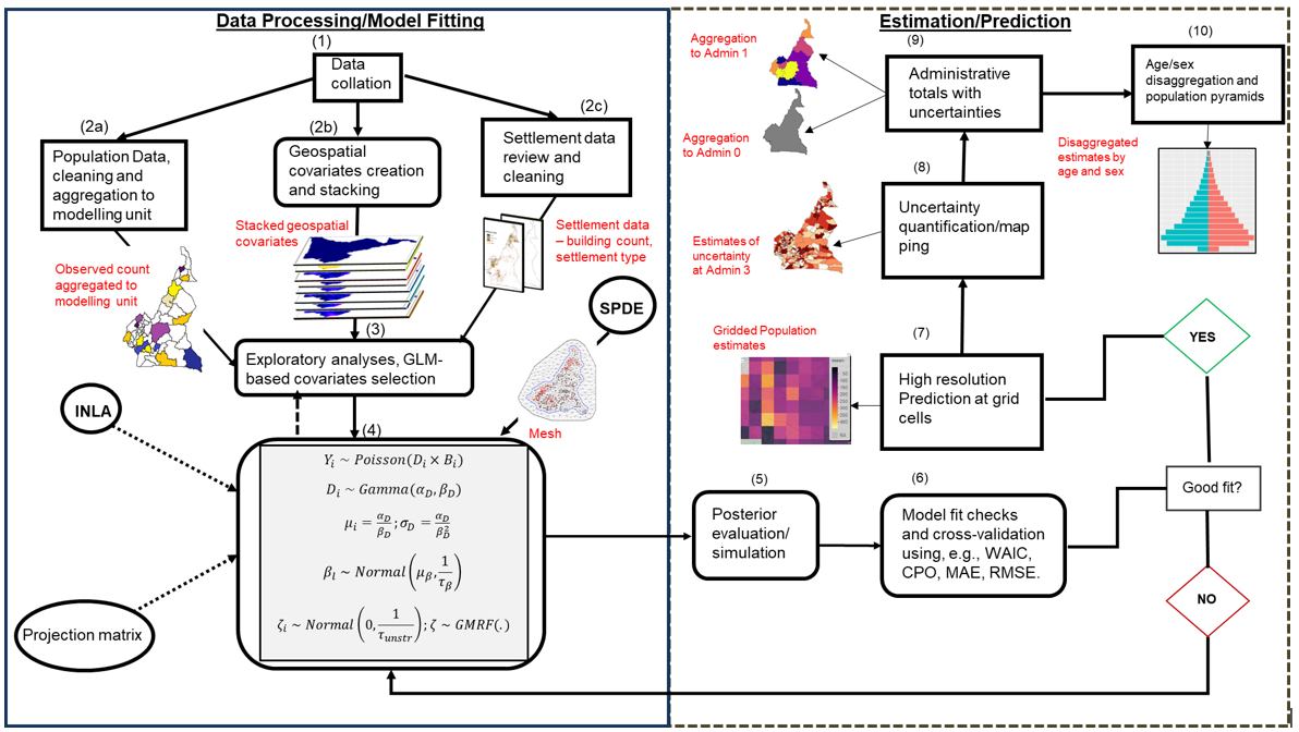
Figure 15.1: A schematic representation of the workflow of INLA-SPDE based bottom-up population modelling framework. Note: WAIC – Widely Acceptable Information Criterion; CPO – Conditional Predictive Ordinate; MAE – Mean Absolute Error; RMSE – Root Mean Square Error.
As illustrated in Figure 15.1, input datasets are first assembled from the various sources and then prepared and cleaned for population estimation. The data preparation activities in step 2 also includes the processing of key geospatial covariates (nighttime light, distance to marketplace) and settlement data (e.g., building footprint, residential status) that could influence population distribution. The combined population datasets are then used in step 3 to construct a generalized linear model (GLM) which identifies the geospatial covariates that significantly predict population distribution. Step 4 involves the implementation of Bayesian statistical model using INLA-SPDE (integrated nested Laplace approximation – stochastic partial differential equations). INLA-SPDE provides computational efficiency by using the mesh which is a triangulation of the entire spatial domain of interest instead of modelling a computationally expensive continuous space, and then projects the observations at the mesh nodes using the projection matrix (more details of the INLA-SPDE implementation are provided in chapter 16. Steps 5 to 10 follow immediately after model fitting and involves the collation and testing of the model results, high resolution (approximately 100 m by 100m) prediction at grid cell levels, aggregation to various administrative units of interest, and disaggregation of the population totals at various age/sex strata.
A detailed modelling framework of geostatistical modelling of population estimates has been provided in chapter 16. In summary given a set of population count and geospatial covariates, the hierarchical regression modelling framework is of the form
\[\begin{equation*} population = \frac{people}{building}\times building\tag{8.1} \end{equation*}\]
where the first term, number of people per building, is the population density, \(D\). Note that the ‘building’ in equation (1) (8.1) can be any covariate that sufficiently defines the settlement intensity, e.g., the total built-up area, number of buildings, number of households, building intensity
The population count \(Y_i\) within a given settled area \(i\) is naturally assumed to be a Poisson distributed random variable with the parameter \(\lambda_i\), that is,
\[\begin{equation} Y_i \sim \text{Poisson}(D_i \times B_i)\tag{8.2} \end{equation}\]
where \(D_i\) is the population density which captures the variability in the population data, and \(B_i\) is the (usually satellite observed) settlement (building) intensity. The overdispersion is therefore modelled explicitly via the density parameter by assuming appropriate statistical distribution. A gamma distribution is assumed for population density \(D_i\) and is given as
\[\begin{equation} D_i \sim \text{Gamma}(a_{\gamma}, b_{\gamma}) \tag{8.3} \end{equation}\]
Where \(a_{\gamma}\) and \(b_{\gamma}\) are the shape and rate parameters such that \(E[D_i ]\) = \(\bar{D_i}\) = \(a_{\gamma}\) /\(b_{\gamma}\), \(var(D_i )=a_γ/(b_γ^2 )\), then \(\bar{D_i}\) is linked to the geospatial covariates through the linear predictor \(η(s_i)\) given by
\[\begin{equation} h(\overline{D}(s_i)) = \eta(s_i) \tag{8.4} \end{equation}\]
the full model used in this study is of the form:
\[\begin{equation} \eta(s_i) = \beta_0 + \sum_{k=1}^K \beta_k x_{i,k} + \sum_{m=1}^M f_m(z_{m,i}) + \sum_{h=1}^H \tilde{A}_{ih} \zeta + f_p(\text{type}) + f_r(\text{reg}) + f_{r,p}(\text{reg} \times \text{type}) + \epsilon_i \tag{8.4} \end{equation}\]
where \(\beta_0\) is the intercept parameter representing the average population density when there is zero effect of the other covariates; \((β_1,…,β_K )\) are the unknown fixed effect coefficients of the K geospatial covariates \((x_1,x_2,…,x_K )\) found to significantly predict the population density; \(\epsilon_i\) is a Gaussian noise or nugget effect (Cressie 2015), which accounts for the observation level variability, also known as the fine scale variability, (e.g Paige et al. 2022) not captured by the geospatial covariates, that is \(\epsilon_i∼Normal(0,σ_\epsilon^2 )\), \(\{f_m\}_{m=1}^M\) are the random effect functions of the \(M\) different data sources; while \(f_p (type)\), \(f_r (reg)\), and \(f_{r,p}(reg×type)\) capture the variabilities due to differences in population distributions across different settlement types, regions, and their interactions, respectively. The hierarchical modelling framework allows the incorporation of as many random effects as possible, however, care must be taken to avoid overfitting the data.
The predicted population density \(\hat{D}(s_i)\) is obtained as the back transformed values of the predicted linear predictor \(\hat{\eta}_i\), that is \[\hat{D}(s_i) = \exp(\hat{\eta}_i)\] Finally, the predicted population count is given as a weighted product of the population density and the building count, that is \[\hat{y}_i = \hat{D}_i \times B_i\]
15.3 Simulation Study
15.3.1 Model parameter values and sample sizes
To demonstrate how our methodology works and investigate the potential effects of the differences in the spatial scales of the modelling and prediction units, models were fitted and assessed for a combined total of 40 datasets simulated based on various permutations of the parameters in Figure 15.2
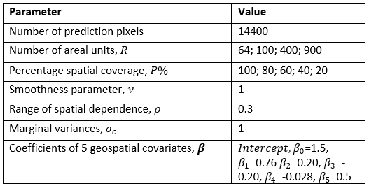
Figure 15.2: Data simulation sample sizes and initial model parameters.
Specifically, we simulated data for \(G = 14400\) prediction square grid cells. These grid cells were then grouped under \(R\) equally sized nonoverlapping area units such that each area unit contains \(g=G/R\) grid cells, where \(R\) takes values from \(\{64,100,400,900\}\) (see Fig. 15.3) below. \(R=100\) with \(g=144\) grid cells per square area). However, we assume that observations within areas that are neighbours share some characteristics which would be exploited in parameter estimation. To fully explore the potential impacts of sample size on model predictions, data are allowed to be either fully observed (no missing data) or have a given proportion P of the entire grid cells observations missing uniformly at random where P takes values from \(\{100\%, 80\%, 60\%, 40\%, 20\%\}\). For example, Figure 15.3B shows the mesh of the grid cells observations for \(R=100\) area units with only the \(P= 40%\) of the entire grid cells observations available. Thus, in this case, model will be trained using the 40% of the entire grid cell data and the estimates used to predict values for the 60% grid cells not observed.
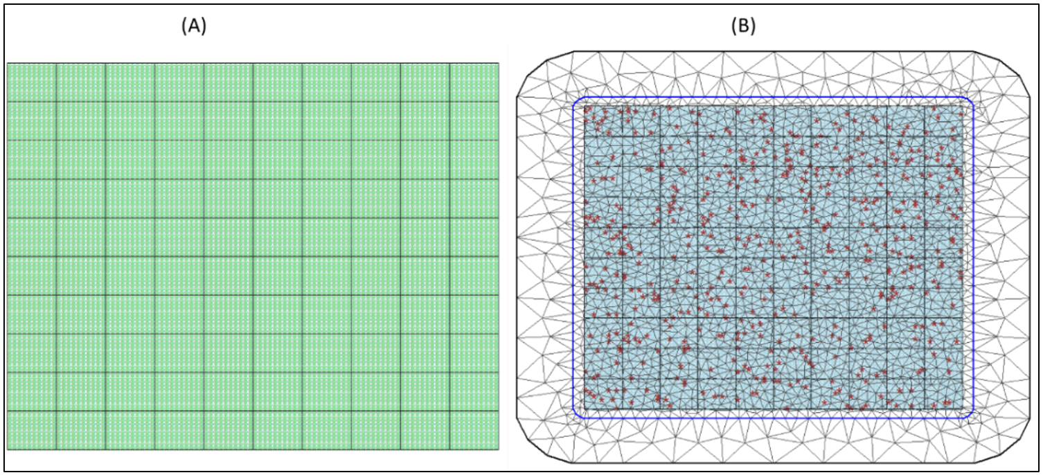
Figure 15.3: (A) 14400 prediction grid cells distributed equally across 100 regular square areal units such that each area unit contains 14400/100=144 grid cells, and (B) A triangulation mesh overlayed over the entire spatial domain. The red points are the 40% of the grid cells with observations. Note that the number of observed grid cells (red) varies randomly across the area units (Figure 3B).
Moreover, there are 5 datasets for each of the \(R\) area units data with \(P \in \{100\%, 80\%, 60\%, 40\%, 20\%\}\) coverage, so that there is a total of 20 datasets across all the \(R \in \{64, 100, 400, 900\}\) spatial units. In addition, data are aggregated at the area level for each of the 20 datasets to obtain the corresponding areal-level data, thus, making it 40 datasets in all (20 grid cell-level, 20 aggregated areal-level). The motivation for this areal-level aggregation is to examine the effects of the percentage coverage (sample size) on the prediction accuracies under two scenarios:
- Grid2Grid: This is when parameters are estimated at grid cell level and predictions also made at grid cell level.
- Area2Grid: This is when data are aggregated at areal level with parameters estimated at the areal level while predictions are made at grid cell level.
Spatial autocorrelation parameters based on the Matérn covariance structure for INLA-SPDE (see equation 7 of chapter 16) were also chosen such that the smoothing parameter \(ν=1\); range of spatial dependence \(ρ=0.3\), and marginal variance \(σ_c=1\). These parameter choices yield a scale parameter value of \(κ =√(8×1)/0.3\) which depends only on the spatial dependence parameter \(ρ\).
15.3.2 Geospatial Covariates and Random Effects
In Figure 15.4, we present the distribution of the geospatial covariates and other random effects simulated for this study. Although the probability distributions from which the geospatial covariates are drawn are arbitrary, we ensured that the values are within reasonable range of values for such covariates often used in a real data population modelling setting. Spatial autocorrelation was implied through distance dependent precision matrix \(Q\) so that the spatially correlated random effect is a Gaussian Markov Random Field (GMRF, Lindgren et al. 2011).
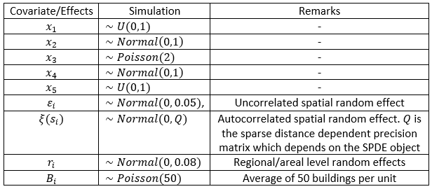
Figure 15.4: Simulation of geospatial covariates and random effects.
Regional/areal level random effects are simulated as \(r_i∼Normal(0,0.08)\), where the variance of 0.08 is chosen based on some initial analyses. This ensures that the variability due to unobserved areal units differences including spatial misalignments are accounted for. Finally, the building count variable is simulated as \(B_i∼Poisson(50)\) assuming that on average, there are 50 buildings in each prediction unit.
15.3.3 Estimating the mean of the population density
The simulated geospatial covariates and the random effects are then used to obtain the mean of the population density \(μ(s_i)\) according to Equation (8.5) below
\[\begin{equation} \ln(\mu(s_i)) = \beta_0 + \beta_1 x_1 + \beta_2 x_2 + \beta_3 x_3 + \beta_4 x_4 + \beta_5 x_5 + \xi(s_i) + r_i + \epsilon_i \tag{8.5} \end{equation}\]
Then, in line with Equation (8.4), we simulate the population density using
\[\begin{equation} D_i \sim \text{Gamma}\left(\frac{\hat{\mu}(s_i)^2}{\phi}, \frac{\hat{\mu}(s_i)}{\phi}\right) \tag{8.6} \end{equation}\]
where \(\hat{\mu}\) and \(\phi\) are the estimated mean and the variance of the population density, respectively; \(β_0\) and \(β_1, …,β_5\) are the intercept and fixed effects coefficients of the geospatial covariates \(x_1,…,x_5\) listed in Figure 15.4, respectively. Here we set \(\phi = 0.01\), and \(\hat{\mu}̂(s_i)=exp(\mu(s_i)\), the back transformed average population density. Finally, the population count for each grid cell is obtained as
\[\begin{equation} \mathbf{y}_{ga} \sim \mathrm{Poisson}(D_i \times B_i) \tag{8.7} \end{equation}\]
where \({y}_{ga}\) is the count of people in the \(g\)th grid cell of area \(a\) \((a=1, …, R; g=1, …,n_a)\). In the next Section, we provide a step-by-step detail of the data simulation processes.
15.3.4 Data Simulation
First, as illustrated in Figure 15.2, we created \(G=14400\) grid cells over a unit area divided into \(R\) sub-area units such that there are \(g\) equal number of grid cells within each sub-area \(a\) \((a=1,…,R)\). Next, we simulate data for all the grid cells by first assuming that the population is fully observed, that is, \(P=100\%\). Then, we aggregate the grid level datasets to the corresponding areal units according to Equation (8.8) to Equation (8.10) below. All the simulation codes are provided here simulation code.
Areal level aggregation of observed data and geospatial covariates
- Count: The count for the \(a\)-th area is the total count of people for all the grid cells belonging to area \(a\), that is
\[\begin{equation} y_a = \sum_g y_{ag} \tag{8.8} \end{equation}\]
where \(y_{ag}\) is the number of people ‘observed’ in the \(g\)-th grid cell of area \(a\).
- Building: Similarly, the number of buildings in area \(a\) is obtained by adding all the buildings in all the grid cells that fall under area \(a\) together, that is,
\[\begin{equation} B_a = \sum_g B_{ag} \tag{8.9} \end{equation}\] where \(B_{ag}\) is the number of buildings ‘observed’ in the \(g\)-th grid cell of area
- Geospatial Covariates: The corresponding areal level estimates of the geospatial covariates is obtained as the average value of the covariates across all the grid cells in area \(a\). Thus
\[\begin{equation} x_a = \frac{1}{n} \sum_{g=1}^n x_{ag} \tag{8.10} \end{equation}\]
where \(x_{ag}\) is the value of a given geospatial covariate in the \(gth\) grid cell of area \(a\). Once datasets are sorted for both areal and grid cell levels, the model specified in Equation (8.5) is fit separately to the areal level aggregated data and to the Grid cell level data. Model predictions at the grid cell levels are then made with the best fit models. By allowing the entire grid cells to be fully observed, it provides the opportunity for direct model validation by comparing the grid cell predictions with the observations. Our focus is on assessing how accurate the areal unit model-based predictions would be compared to the grid cell level model predictions. In particular, we repeated the processes for the various sample sizes and coverage percentages listed in Figure 15.2.
When data are fitted at the grid cell level and prediction made at the grid cell level, we call this the Grid-to-Grid or Grid2Grid approach. But when data are fitted at the areal level and predictions are made at the grid level, we call this Area-to-Grid or Area2Grid.
15.3.4.1 Data Simulation Steps
- Specify the initial parameter values as given in Tables 1 & 2:
- Do the following for each number of areal units and percentage coverage combinations:
Grid-to-Grid (Grid2Grid)
Simulate the geospatial covariates and the response variable (the number of people in each grid cell) over the entire prediction grid cells (\(G=14400\)) across all the areal units.
Fit the model at the grid cell level.
Predict population and estimates of uncertainties at the grid cell level which is briefly highlighted below:
- Run posterior simulations based on the initial model posterior distribution using the inla.posterior.sample() function to generate a sampling distribution of the posterior means.
- If required, aggregate the posterior samples to the areal unit of interest to form the sampling distribution of the totals at the given areal unit.
- For each set of the posterior samples, obtain the desired sample statistics such as the mean, standard deviation and 95% quantiles from the posterior samples.
Area-to-Grid (Area2Grid)
- Fit the model at the areal unit level using exactly the same model specifications used at the grid cell level to account for the differences in the spatial resolutions and also to ensure the comparability of the estimates.
- Using the areal levels estimates make predictions at the grid cell level by repeating the processes outlined in step 5 above, and obtain the aggregated estimates based on the areal level estimates.
- Repeat steps 3 to 7 until the desired number of scenarios are obtained.
15.3.5 Model fit checks and cross-validation
To assess the model, model goodness-of-fit, cross-validations and model prediction performance checks were based on a constellation of metrics. Specifically, we used the Widely Applicable Information Criterion (WAIC, Watanabe 2013) and Conditional Predictive Ordinate (CPO, Pettit 1990) for model fit assessment and cross-validation, respectively. For model predictive ability, we used Mean Absolute Error (MAE), Root Mean Square Error (RMSE) and the Pearson Correlation or scatter plots of observed versus predicted. The WAIC measures the goodness-of-fit of a model based on the complexity of the model such that smaller WAIC value indicates a better fit.
15.3.6 Simulation Study Results
Overall, the Grid2Grid model predictions were more affected by proportion of missing values rather than the number of area units, while the model performance metrics results for Area2Grid model predictions are somewhat mixed and suggest that the Area2Grid models are affected by the combined effects of missingness and sample size (Figure 15.5).Similar trends of the model performance indices estimate based on MAE and RMSE were obtained for the Grid2Grid models (Figure 15.5A and Figure 15.5C). These show that the Grid2Grid models performed worse as the proportion of missing data increased with larger sample sizes most affected by number of missing values. The result is somewhat expected in that higher proportion of missing values for a larger sample size would mean higher number of missing samples when compared with smaller samples with the same proportion of missing values. On the other estimates of MAE and RMSE metrics for the Area2Grid model, (Figure 15.5B & Figure 15.5D) show similar trends, however, Figure 15.5D shows that the model performed worse for n=900 area units when only RMSE values are considered. It should be noted that although both RMSE and MAE measure magnitude of error, MAE measures the average magnitude of errors in predictions while RMSE errors are first squared before they are averaged (see equations 27 and 28 of Chapter 16). Thus, the values of RMSE are always higher than that of MSE.
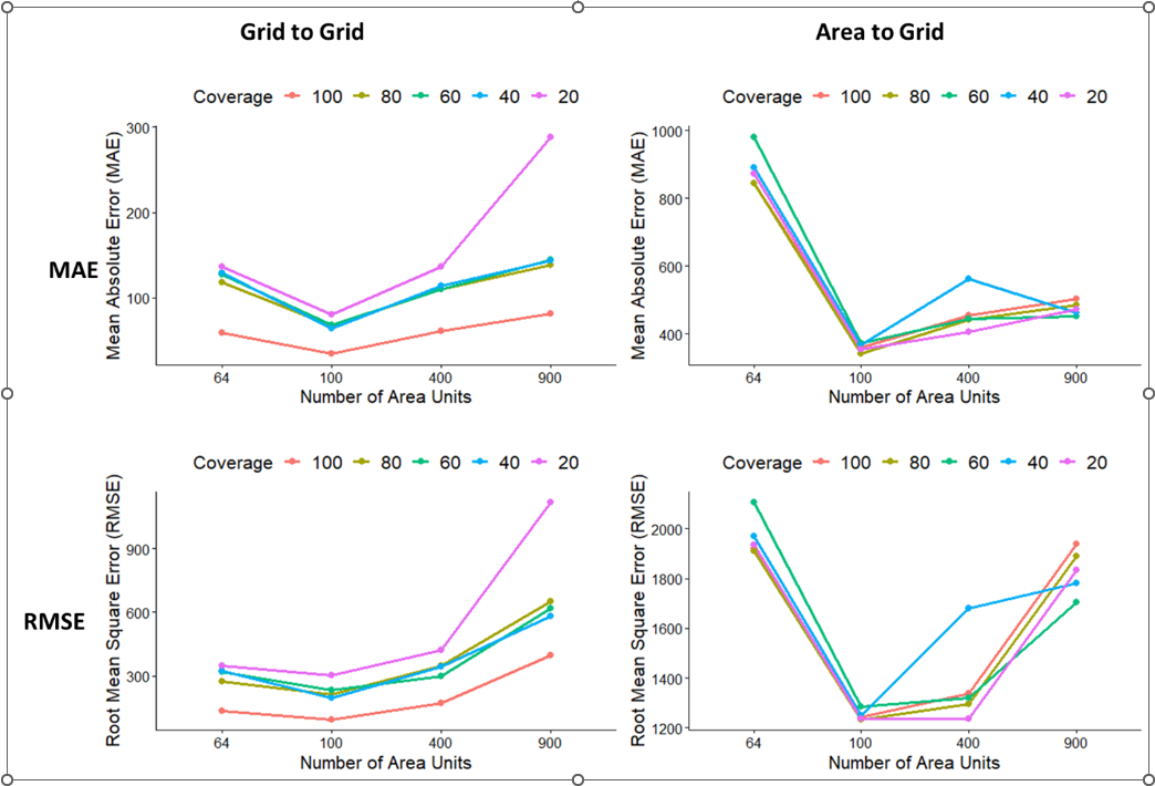
Figure 15.5: Estimates of the MAE and RMSE values of the models across various levels of missing values for Grid2Grid and Area2Grid models.
Moreover, model cross-validation metrics based on the CPO suggest that the model performance improved as more data are observed (less proportion of missing values) for larger number of area units (sample size) for both Grid2Grid and Area2Grid models (Figure 15.6). In addition, the posterior estimates of the total population counts compared across the various sample sizes and percentage coverages for Grid2Grid and Area2Grid models indicate that Area2Grid models predictions more closely approximates Grid2Grid estimates as the number of area units (sample size) increased even when only 20% of the entire grid cells are observed (see Table S2.1 – Table S2.4 of the of the supplementary document which can be found here supplementary materials
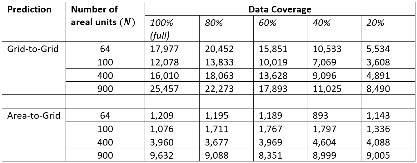
Figure 15.6: CPO values of the best fit models fitted to the Grid2Grid and Area2Grid datasets.
Posterior density plots of the log predicted population counts across the various sample sizes – percentage coverage combinations for the Grid-to-Grid models overlaid with the corresponding Area-to-Grid estimates, is shown in Figure 15.7.Results show that the posterior distributions were dissimilar over small sample sizes (R≤100 area units) with the Area-to-Grid models performing worse, but these quickly improved as the sample sizes became larger (R≥400 area units). Estimates of the predicted posterior spatial random effects (Mean and SD) are shown in Figure S2.1 of the supplementary materials.
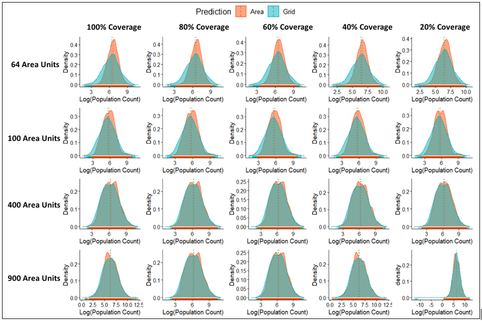
Figure 15.7: Comparisons of the posterior density plots of log of the predicted population counts across the various sample size-spatial coverage combinations for Grid-to-Grid versus Area-to-Grid models. Predictions based on the Area-to-Grid models become more similar to that of the Grid-to-Grid models as the sample size increases irrespective of the amount of missing data.
In Figure 15.8, we compared directly grid cell level predictions of the Area-to-Grid models versus Grid-to-Grid models using scatter plots and we found that the Area-to-Grid predictions performed worse for small samples but both predictions became more in agreement with a correlation coefficient of ~95% as the sample sizes increased.
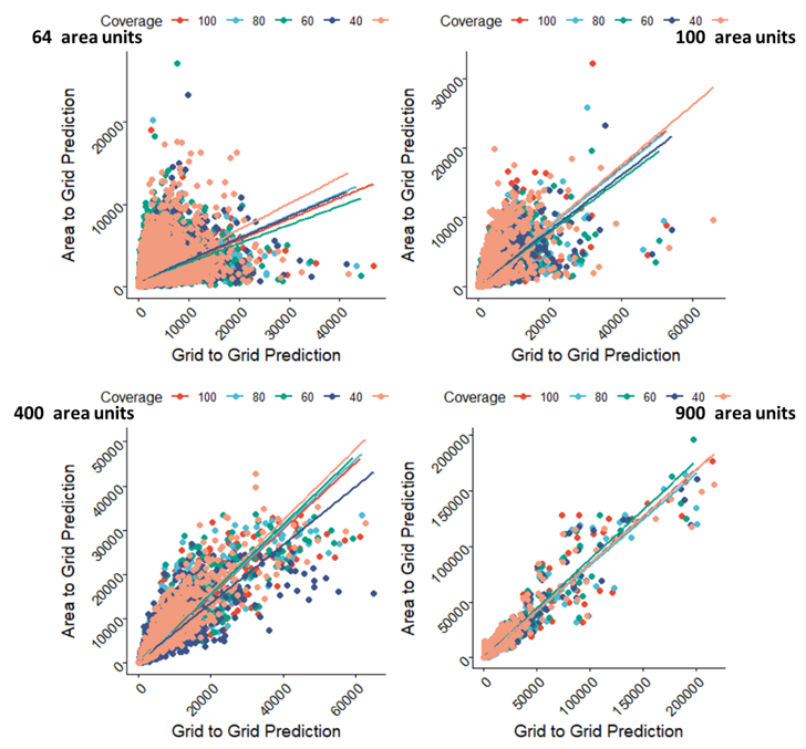
Figure 15.8: Comparisons of the scatter plots of the Grid-to-Grid models prediction versus the Area-to-Grid models predictions across the various sample size-spatial coverage combinations. Predictions based on the Area-to-Grid models become more similar to that of the Grid-to-Grid models as the sample size increases irrespective of how much data are missing.
Similarly, the scatter plots in Figure 15.9 compares the predicted counts with the observed counts across the different data scenarios. Throughout, as expected, the Grid-to-Grid predictions showed high positive correlations (correlation coefficient > 0.98) with the observed counts. On the other hand, at \(R=64\) area units, the Area-to-Grid predictions performed worse and varied across various percentage coverages as well. However, as sample sized increased, the predictive ability of the Area-to-Grid models quickly improved especially for 400 and above area units irrespective of the proportion of missing data. See also Figures S2.2 and S2.3 in the supplementary materials for the corresponding scatter plots for the aggregated area totals based on the Grid-to-Grid versus the Area-to-Grid models.
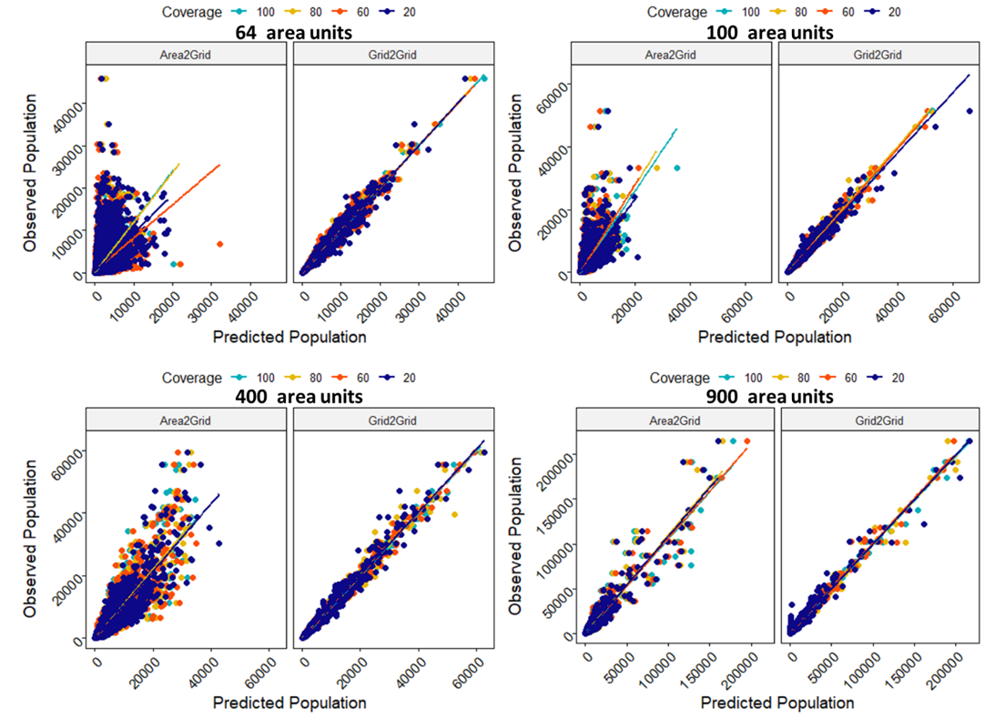
Figure 15.9: Comparisons of the scatter plots of the Grid-to-Grid models prediction versus the Area-to-Grid models predictions across the various sample size-spatial coverage combinations. Predictions based on the Area-to-Grid models become more similar to that of the Grid-to-Grid models as the sample size increases irrespective of how much data are missing.
In Figure 15.10, we compare the spatial distributions of the log of the predicted population means based on the Grid-to-Grid and Area-to-Grid models across the grid cells and area units across various number of area units. The maps support the earlier findings that as the sample size becomes larger, Area-to-Grid models provide good approximations to the Grid-to-Grid model predictions in that the spatial patterns are almost identical irrespective of the amount of missing data.
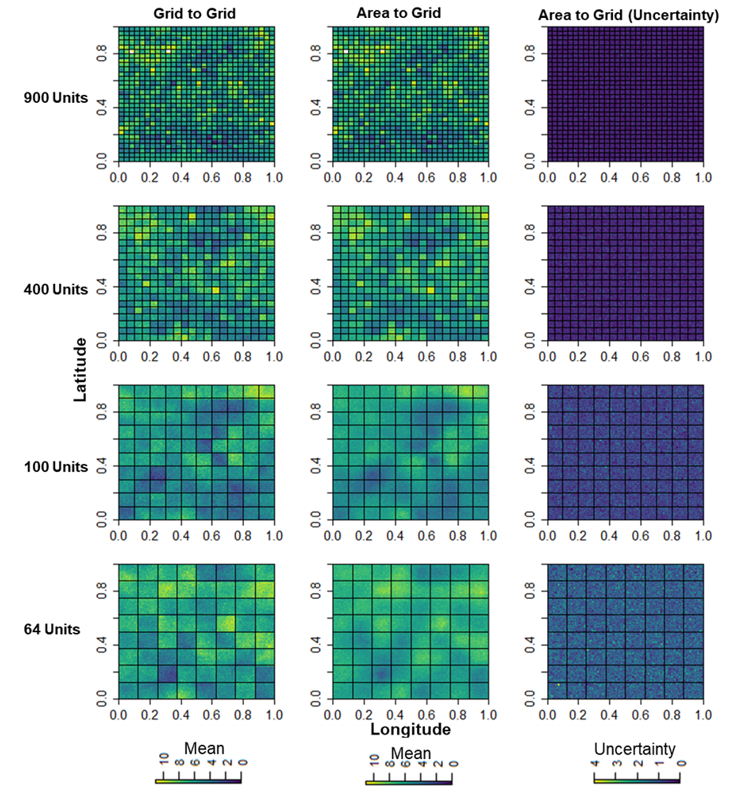
Figure 15.10: Spatial distribution of the log posterior means for the Grid-to-Grid versus Area-to-Grid models across the various number of area units. Uncertainty increased as the number of area units decreased.
Also, the maps in Figures 15.10 and 15.11 show the log of the mean posterior predictions across the various area units-percentage coverage combinations along with the uncertainty maps based on the Area-to-Grid predictions only. The models predictions performed well across all levels of missingness but performed poorly with higher uncertainty for smaller number of area units.
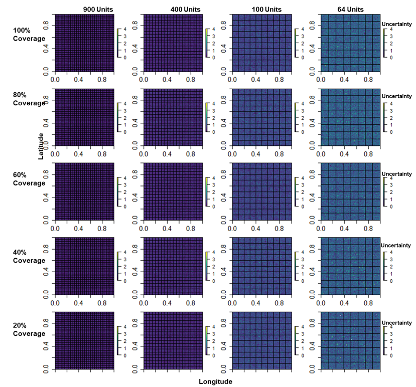
Figure 15.11: Uncertainty maps of the predicted population count across the various number of area units - coverage combinations (Area to Grid predictions only). Posterior estimates of uncertainty increased as the number of area units decreased, thus, models with smaller number of area units have the highest level of uncertainty in their parameter estimates, but the level of missing had only limited impact on the results.
15.4 Application to Cameroon Household Listing Datasets
As a proof of concept, in this Section, using five household listing datasets, we show how our methodology could be used to produce estimates of population numbers at various administrative units in Cameroon.
15.4.1 Input Datasets
In all, there were 2587569 counts of people across 509628 households contained within the 2290 Enumeration Areas (EAs) in the cleaned five household listing datasets as shown in Figure 15.12, which translates into a national average of ~5 people per household. These model input datasets obtained from the Cameroon National Institute for Statistics (NIS) were collected between 2021 and 2022 based on a 2-stage stratified sampling design in which the sampling frame consisted of the list of all households within the EAs selected in the first draw. Other datasets obtained from the NIS are administrative boundaries shapefiles.
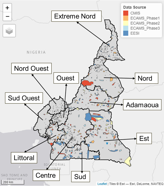
Figure 15.12: Map of Cameroon showing the distribution of the 2290 Enumerations Areas (EAs) observed within the 5 household listing datasets. CMIS - Cameroon Malaria Indicator Survey (CMIS 2022); ECAMS_Phase1-The 2021/2022 fifth Cameroon Households Survey phases 1; ECAMS_Phase2-The 2021/2022 fifth Cameroon Households Survey phases 2; ECAMS_Phase3-The 2021/2022 fifth Cameroon Households Survey phases 3; EESI - Employment and Informal Sector Survey.
15.4.2 Bayesian Hierarchical Modelling
15.4.2.1 Covariate Selection
Prior to model fitting, the covariates were scaled based on the z-score in Equation (8.6) and we used a GLM-based stepwise covariates selection methods according to Equation (8.5) implemented in R via the stepAIC() function of the ‘MASS’ package with the selection direction option set as ‘both’. In addition, covariates chosen in step 1 are further checked for multicollinearity using the ‘vif’ function of the ‘car’ package. As a rule of thumb, covariates with vif values less than \(5\) were deemed acceptable and therefore retained, while those with vif values greater than \(5\) were dropped (James et al. 2013). In Figure 15.13, we present the attributes of the 8 geospatial covariates that were eventually chosen and retained out of the 43 covariates initially considered for the final models specification and parameter estimations.
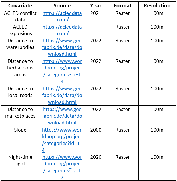
Figure 15.13: List of the last 8 geospatial covariates included in the final model.
Like the simulation study geospatial covariates, these covariates in Figure 15.13, represent the averages of the grid cell values for the corresponding EA extracted based on the master grid of Cameroon.
15.4.2.2 Model Implementation Within INLA-SPDE Framework
The triangulation mesh used in the model contains 534 nodes (see Figure S3.1) of supplementary materials where the observations are projected via the projection matrix. Also, similar to the areal unit level of the simulation study, the centroids of the EAs are used for the mesh construction.
To account for aggregation error, we assume that the observed count in the household listing datasets are Poisson distributed as specified in Equation (8.2) to Equation (8.4) as
\[\begin{equation} Y_i \sim \text{Poisson}(D_i \times B_i) \end{equation}\]
\[\begin{equation} D_i \sim \text{Gamma}(a_{\gamma}, b_{\gamma}) \end{equation}\]
\[\begin{equation} \text{where} \; E[D_i ] = \bar{D_i} = a_{\gamma}/b_{\gamma} \end{equation}\]
\[\begin{equation} h(\overline{D}(s_i)) = \eta(s_i) \end{equation}\]
For this application the settlement data used is the building number within a given EA. This was used to calculate the population density prior to the model fitting.
In total, four nested models specified below were further tested within a Bayesian inference framework. Note that initial models included the random effect term to account for potential variabilities due to any differences in data collection methods. However, the initial models suggested that the data source random effect could be dropped. Model assessment and model fit selection are based on the model fit indices outlined in (model fit checks) section.
\[\begin{equation} Model\text{ } I: \eta(s_i) = \beta_0 + \sum_{k=1}^8 \beta_k x_{i,k} + \sum_{d=1}^{534} \tilde{A}_{id} \zeta + f_p(\text{type}) + \epsilon_i \end{equation}\]
\[\begin{equation} Model\text{ } II: \eta(s_i) = \beta_0 + \sum_{k=1}^8 \beta_k x_{i,k} + \sum_{d=1}^{534} \tilde{A}_{id} \zeta + f_p(\text{type}) + f_r(\text{reg}) + \epsilon_i \end{equation}\]
\[\begin{equation} Model\text{ } III: \eta(s_i) = \beta_0 + \sum_{k=1}^8 \beta_k x_{i,k} + \sum_{d=1}^{534} \tilde{A}_{id} \zeta + f_{r,p}(\text{reg} \times \text{type}) + \epsilon_i \end{equation}\]
\[\begin{equation} Model\text{ } IV: \eta(s_i) = \beta_0 + \sum_{k=1}^8 \beta_k x_{i,k} + \sum_{d=1}^{534} \tilde{A}_{id} \zeta + f_p(\text{type}) + f_{r,p}(\text{reg} \times \text{type}) + \epsilon_i \tag{8.11} \end{equation}\]
where, the terms \(\beta_0\), \(\{\beta_k\}_{k=1}^8\), \(A\), \(\zeta\), \(f_p\), \(f_{r,p}\), and \(\epsilon\) are intercept, fixed effect coefficients of the 8 geospatial covariates, projection matrix, spatial autocorrelation term, settlement type,settlement type – region interaction term, and the zero mean Gaussian nugget effect.
Following from some initial sensitivity analyses using various choices of priors and hyperpriors values, the following INLA default priors and hyperpriors were assigned to the parameters and hyperparameters:
\[\begin{equation} \beta_0 \sim Uniform(0,1) \end{equation}\]
\[\begin{equation} \beta_k \sim Normal(0,0.01) \end{equation}\]
\[\begin{equation} \theta \sim Normal(0,1000), \text{where} \; \theta \in \{f_m,f_p,f_{rp}\} \end{equation}\]
\[\begin{equation} \tau_\epsilon \sim Gamma(0.01,0.01) \end{equation}\]
\[\begin{equation} \tau_w \sim Gamma(1,0.00005) \text{ where} \; \text{w} \in \{\beta,m,p,rp\} \tag{8.12} \end{equation}\]
Note that instead of the weakly informative priors utilised here, a joint penalized complexity (PC) prior (Fuglstad et al. 2019) could still be used.
Finally, the predicted density \(\hat{D}_i\) of a given spatial unit (enumeration area) is obtained as the exponential of the linear predictor, that is,
\[\begin{equation} \hat{D}_i = \exp(\hat{\beta}_0 + \sum_{k=1}^8 \hat{\beta}_k x_{i,k} + \sum_{d=1}^{534} \tilde{A}_{id} \zeta + \hat{f}_p (\text{type}) + \hat{f}_{r,p} (\text{reg} \times \text{type}) + \hat{\epsilon}_i) \tag{14.1} \end{equation}\]
Then, the predicted population count is obtained using \(\hat{y}_i=\hat{D}_i \times B_i\)
15.4.3 Results
Application to the real-life modelling results is presented in this Section.
15.4.3.1 Model fit metrics
With respect to the model assessment metrics in Figure 15.14 below, Model IV which has the lowest WAIC and lowest CPO values provided the best fit for the data.
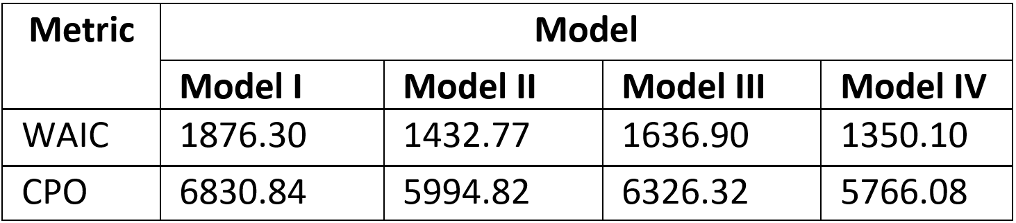
Figure 15.14: Model fit indices for the top competing models.
15.4.3.2 Proportion of variance explained
To estimate the proportion of the variability within the observations that are attributable to the correlated spatial random effects, with a view to further justifying the inclusion of the spatial autocorrelated term within the model, we evaluated the posterior precision as \(\tau_\zeta =0.152\) of the best fit model (Model IV) using marginal.variance.nominal option of the R-INLA package. Also, the posterior precision of the uncorrelated spatial random effect was evaluated as \(\tau_\epsilon = 2.771\) via \(summary.hyperpar\) evaluation option. Thus, the proportion of the total variance explained by the correlated spatial random effects (Model IV) is given by
\[\hat{\zeta} = \frac{\sigma_{\zeta}^2}{\sigma_{\zeta}^2 + \sigma_{\epsilon}^2} = \frac{6.598}{6.598 + 0.361} = 0.948\]
where \(\sigma_q^2=1/\tau_q\) and \(q \in \{\zeta,\epsilon\}\).This indicates that the inclusion of the spatial random effects allowed us to account for nearly 95% of the total variability in the data thereby unmasking and decomposing spatial effects due to spatial autocorrelation from those due to spatial independence, thereby greatly minimizing estimation biases.
15.4.3.3 Cross- Validation
In addition to the leave one out cross validation already performed across models, we carried out further cross validation of the identified best fit model. Specifically, a k-fold cross validation was used to test the stability and the predictive ability of the model. Here, the data are randomly divided into in 20% test set and 80% train set for each k fold (k=5). For each fold, the 80% train set is used to train the model while the test set is used for prediction. Model fit metrics and correlation (scatter) plots are produced for each non-overlapping test sets. Figure 15.15 below provide results of the test. Further validation results can also be found in (Table S3.1, Figure S3.2) of the supplementary materials
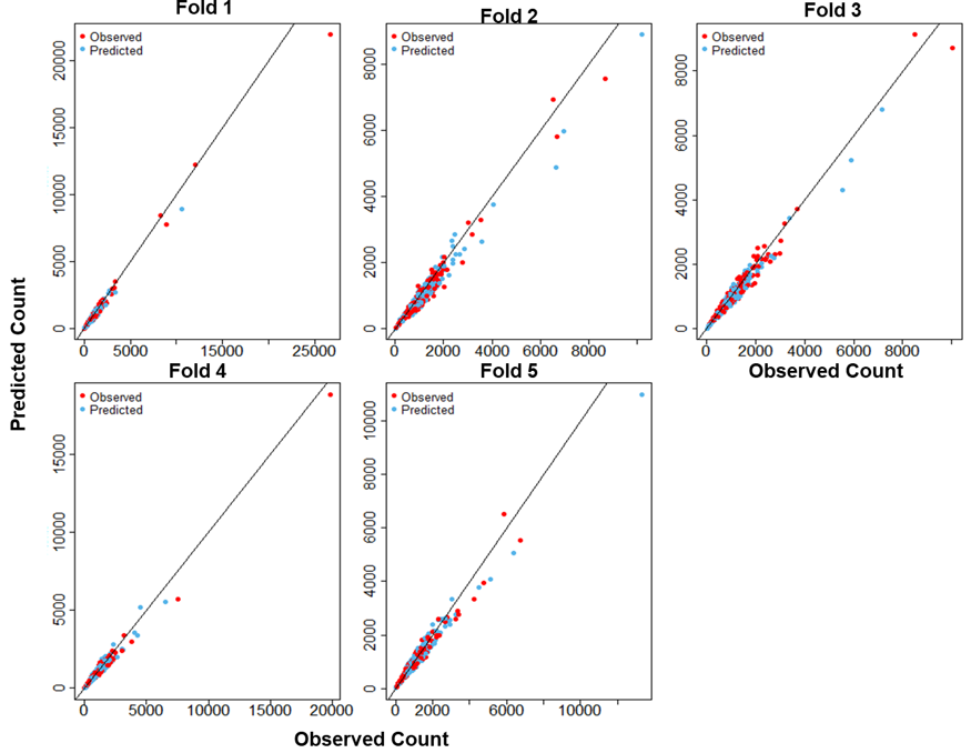
Figure 15.15: Scatter plots of the posterior cross-validation predictions of the Cameroon data model versus the observed data across the k=5 folds.
15.4.3.4 Fixed Effects Coefficients
The posterior estimates of the fixed effects coefficients are provided in Figure 15.16. As these covariates are Z-score transformed, they are interpreted in terms of standard deviation. For examples, the results show that the standard deviation of the population density will increase by 0.068 for any unit increase in the standard deviation of night-time light. Also, the results indicate that for any unit increase in the standard deviation of the slope, the standard deviation of the population density decreases by 0.0891 units.
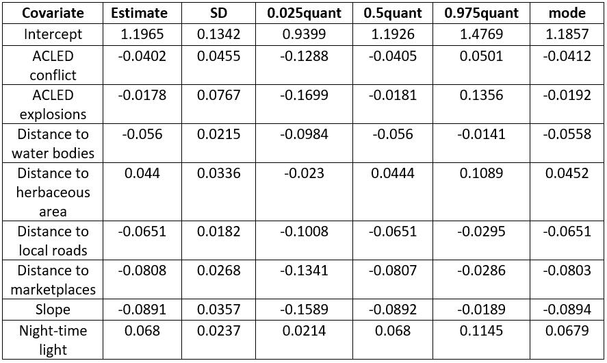
Figure 15.16: Posterior estimates of the fixed effects of the best fit model.
15.4.3.5 Comparison Between INLA-SPDE Estimates and NIS Projections at Admin 1
Estimates of population at Admin level 1 from our methodology were compared with the NIS Projections Admin 1 for 2022 (National Institute of Statistics 2016). NIS projections are produced using cohort component methods that do not account for changes occurring over the time period of projection, nor at small area scales. One of the advantages of the modelling approach outlined here is that it takes advantage of more recent small area population data that can capture such changes. We therefore do not expect our modelled estimates to agree with the projections perfectly, however, it is interesting to note from Figure 15.17 that both estimates are in agreement with each other for about 70% of the time.
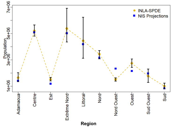
Figure 15.17: Comparison of WorldPop modelled estimates versus NIS Census Projections for Admin 1 in 2022. The black error bars represent the associated 95% credible intervals with the lengths corresponding to the width of the uncertainties.
One key strength of our methodology is the ability to use areas with observations to predict population in areas where little or no data exists. Figure 15.18 shows the spatial distribution of the observed data, the prediction, and the uncertainty at Admin 3 level. There were clusters of people in high cities such as Douala and Littoral regions.
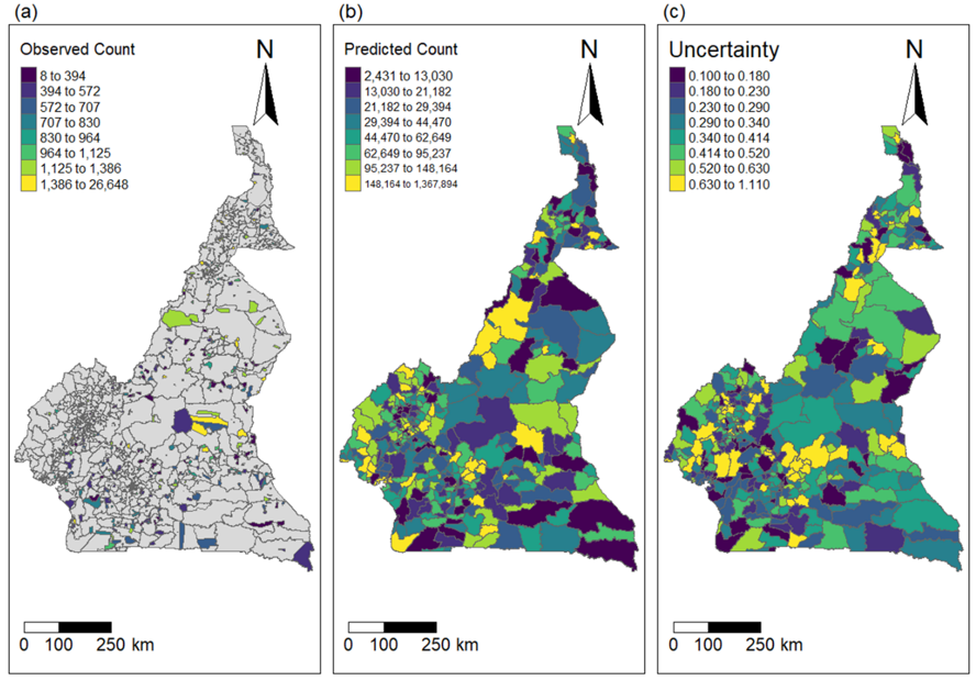
Figure 15.18: Spatial distribution of the observed counts, predicted counts and the uncertainty across Admin level 3 in Cameroon. Uncertainty = (Upper - Lower)/Mean.
15.4.4 Discussion
Model-based methods of population estimation are gaining popularity to address gaps and limitation in population data collection. However, there remain potential sources of biases that need to be addressed to ensure accurate estimates and predictions. This includes the discrepancy in spatial scales between statistical modelling units and high-resolution prediction grid cells, which can lead to prediction/aggregation biases. Additionally, spatial autocorrelation within population data needs to be accounted for in population modelling frameworks, and geostatistical models are effective but computationally expensive, hindering their practical implementation. Here we have put forward methods that focus on overcoming these challenges. We have presented an efficient statistical population modelling approach based on the integrated nested Laplace approximation in conjunction with the stochastic partial differential equations (also known as the INLA-SPDE method) (Rue & Held 2005, Lindgren et al. 2011). The INLA-SPDE offers a computationally efficient approach for the integration of multiple data sources and spatial autocorrelation within a coherent Bayesian geostatistical modelling framework. It evaluates the approximate joint posterior distribution of the model parameters \(θ\) and hyperparameters \(ψ\) given the data \(y\), \(π(θ,ψ|y)\) using fast Laplace approximations, and estimates the sparse precision matrix \(Q=Σ^{-1}\) instead of the computationally expensive dense covariance matrix \(Σ\), that is, INLA-SPDE approximates the continuous Gaussian Random Field (GRF) with a sparse discretely indexed Gaussian Markov Random Field (GMRF) through the triangulation of the entire spatial domain. Thus, the methodology explicitly models spatial dependence using a distance-based correlation matrix and improves population prediction by borrowing strength from neighbouring areas with more observations to predict populations in areas with little or no observations.
We carried out a simulation study to investigate the effects of spatial misalignment on the accuracy of the model predictions found large uncertainties in predictions for small samples of area units, but these quickly improved as the sample sizes increased. In addition, we found that our methodology is robust across various proportions of missing values with very limited impact on the accuracy of the population predictions, even when up to 80% of the data are missing.
Our methodology was successfully applied to household listing datasets collected from five nationally representative surveys between 2017 and 2022 in Cameroon. Posterior estimates of population, along with the corresponding 95% credible interval were found to be comparable with the most recent population projections produced by the National Institute of Statistics (NIS) of Cameroon in 2016. The high uncertainty in the posterior estimates of population within the Extreme North region as shown in Figure 15.17 could be due to very low sample sizes in most of the sampling units in the regions (Figure 15.18). To the best of our knowledge, this represents the first INLA-SPDE based Bayesian population modelling approach which investigated the impacts of the differences in spatial resolutions between data observation/modelling unit and population prediction grid cells, using multiple household listing datasets whilst accounting for spatial autocorrelation.
It remains important to note that model-based estimates, such as those explored here, are not inherently more accurate than population census estimates, and should not be seen as a replacement for field enumeration. Bayesian inference allows for the estimation of uncertainties, emphasizing the importance of considering the lower and upper bounds of the estimates in addition to the mean or median values. Under limited resources for field enumeration, these can help to highlight where future collection of population count data could be prioritized to maximally reduce uncertainties. Future research could explore the impact of different numbers of prediction grid cells and the applications to administrative data, such as birth records, in countries with up-to-date high-quality administrative records. Moreover, extensions of the methodology to handle additional sources of data and investigate the impact of different geospatial covariates on population predictions could be explored. Additionally, advancements in computational methods could further improve the efficiency and scalability of the geostatistical modelling approach. Overall, the developed methodology contributes to advancing population estimation techniques, contributes to improving population estimation accuracy and has significant practical implications for health, social care policies, and humanitarian interventions, decision-making and planning.
15.5 Contributions
This chapter was written by Chris Nnanatu with additional support from Ortis Yankey