14 Geostatistical Bottom-Up Modelling
14.1 Introduction
The bottom-up population modelling methods highlighted in the preceding chapters (see chapter 5 to chapter 7) rely on Markov chain Monte Carlo (MCMC) simulations via the STAN statistical software for parameter estimation. STAN uses the Hamiltonian Markov Chain (HMC) updating steps with the No-U-Turn Sampler (NUTS) algorithm (Hoffman & Gelman 2014) which is known to be relatively faster when compared to other MCMC algorithms. However, as with other MCMC algorithms, the issue of model parameters convergence is still not eliminated because estimates of parameters are based on the posterior samples which are believed to correspond to the stationary distributions of the respective Markov chains.
In addition, according to the first law of Geography which states that locations that are close to each other are more similar in characteristics than those that are further apart (Tobler 1970), it is therefore crucial that population estimation models consider the potential influence of spatial autocorrelation in population distribution within a given small area. This important factor is yet to be incorporated within bottom-up population modelling framework.
To address these identified gaps and ensure more accurate posterior parameter estimates, here we introduce an alternative modelling approach based on the Integrated Nested Laplace Approximation method in conjunction with the Stochastic Partial Differential Equation (INLA-SPDE) which is known to be both fast and accurate (Rue et al. 2009).The INLA-SPDE approach evaluates the posterior marginal distribution of the parameters of interest using a deterministic Laplace Approximation technique thus ensuring that the posterior estimates are always reproducible. Furthermore, the use of the SPDE approach ensures an efficient computational gain in that instead of assuming a continuous Gaussian surface, the SPDE allows for discretization of the entire study location into smaller triangles via the mesh, thereby, circumventing the need to carry out several computationally expensive operations involving the dense covariance matrix of the spatially varying random effect (Rue & Held 2005). INLA is thus computationally faster compared to the MCMC (Carroll et al. 2015)
14.2 Model Structure
In general, the population estimate of people in a given area of interest is defined as the number of people within a settled area. In other words,
\[\begin{equation*} population = \frac{people}{building}\times building\tag{8.1} \end{equation*}\]
where the first term, number of people per building, is the population density, \(D\). Note that the ‘building’ in Equation (1) (8.1) can be any covariate that sufficiently defines the settlement intensity, e.g., the total built-up area, number of buildings, number of households, building intensity
The population count \(Y_i\) within a given settled area \(i\) is naturally assumed to be a Poisson distributed random variable with the parameter \(\lambda_i\), that is,
\[\begin{equation} Y_i \sim \text{Poisson}(D_i \times B_i)\tag{8.2} \end{equation}\]
where \(D_i\) is the population density which captures the variability in the population data, and \(B_i\) is the (usually satellite observed) settlement (building) intensity. The overdispersion is therefore modelled explicitly via the density parameter by assuming appropriate statistical distribution. In the context of Nigeria (see chapter 9), (Leasure et al. 2020e) assumed a LogNormal distribution for the population density such that,
\[\begin{equation} D_i \sim \text{logNormal}(\bar{D_i}, \sigma_D^2) \tag{8.3} \end{equation}\]
where \(D_i\) is the log of the expected population density based on a set of geospatial covariates, and \(\sigma_D^2\) captures and quantifies the random variations in the population density due to overdispersion. As noted in (Leasure et al. 2020e), the choice of the LogNormal distribution on the Microcensus data is purely context-specific and followed from a posthoc simulation study.
Apart from the LogNormal distribution, other positively skewed long-tail probability distributions such as the Gamma and Log-logistic distributions could also be used. Following initial model exploration we adopt a gamma distribution for the INLA-SPDE approach. The model is given as
\[\begin{equation} D_i \sim \text{Gamma}(a_{\gamma}, b_{\gamma}) \tag{8.4} \end{equation}\]
Where \(a_{\gamma}\) and \(b_{\gamma}\) are the shape and rate parameters such that \(E[D_i ]\) = \(\bar{D_i}\) = \(a_{\gamma}\) /\(b_{\gamma}\), \(var(D_i )=a_γ/(b_γ^2 )\), then \(\bar{D_i}\) is linked to the geospatial covariates through the linear predictor \(η_i\) given by
\[\begin{equation} ln(\bar{D_i}) = \eta_i = \beta_ {0} + \sum_ {k=1}^ {K} \beta_ {k} x_ {ik} + \varepsilon_i \tag{8.5} \end{equation}\]
where \(β_0\) is the intercept parameter representing the average national population density when there is zero effect of the other covariates; \((β_1,…,β_K )\) are the fixed effect coefficients (to be estimated) of the \(K\) geospatial covariates \((x_1,x_2,…,x_K )\) found to significantly associate with the population density; \(ε_i\) is a Gaussian noise or nugget effect (Cressie 2015), which accounts for the variabilities not captured by the geospatial covariates, that is, \(ε_i∼Normal(0,σ_ε^2 )\).
Previous studies have identified the need to develop population models which account for the variations in population data due to spatial autocorrelation to minimize potential biases in the population estimates due to unobserved spatially varying factors (e.g., Leasure et al. 2020h, Paige et al. 2022). With that in mind, we set to fill this gap and extended Equation (4) (8.4) to include the spatial autocorrelation term \(ξ(s_i )\) so that locations \(s_i∼s_j\) which share common boundaries are more similar to each other in terms of population distribution than those further apart (Tobler 1970). Thus, the spatially varying linear predictor \(η(s_i )\) is given by
\[\begin{equation} \eta (s_ {i}) = \beta_ {0} + \sum_ {k=1}^ {K} \beta_ {k} x_ {ik} + \xi (s_ {i}) + \varepsilon_ {i} \tag{8.6} \end{equation}\]
where \(s_i∈{s_1,s_2,…,s_N }\) is the index of the i-th unit (e.g., Enumeration areas, etc) of the \(N\) geolocated spatial units within the study domain; where \(ξ(s_i )\) is the i-th realisation of the Gaussian Random Field (GRF), that is, \(ξ(s)∼GRF(0,Σ)\), with the distance dependent Matérn covariance function
\[\begin{equation} C(s_ {i}, s_ {j}) = \frac {\sigma_ {\zeta}^ {2}} {\Gamma (\nu) 2^ {\nu - 1}} (\kappa |\lvert s_ {i} - s_ {j}| \rvert)^ {\nu} K_ {\nu} (\kappa |\lvert s_ {i} - s_ {j} \rvert|) \tag{8.7} \end{equation}\]
where \(Γ\) is a gamma function; \(K_ν\) is the modified Bessel function of the second kind, order \(ν\); \(||s_i-s_j ||\) is the Euclidean distance between spatial locations \(s_i\) and \(s_j\); \(ν\) is the smoothness parameter; \(κ=√8ν/ρ\) is the scale parameter where \(ρ\) is the spatial distance at which the correlation is approximately 0.13; \(σ\) is the marginal variance. Within the context of geostatistics, the computation of the dense covariance matrix \(Σ\) becomes very expensive as the sample size increases with a computational cost of \(O(n^3 )\) (e.g., Bakka et al. 2018). However, Rue and Held (2005) showed that the use of the sparse precision matrix \(Q = \Sigma^ {-1}\) which specifies the conditional independence between the random variables offers a huge computational gain (Rue & Held 2005). Using an INLA-based stochastic partial differential approach (SPDE), Lindgren et al. (2011) showed that a further computational gain is achieved specifying the continuously indexed GRF, ξ(s) as a discretely indexed Gaussian Markov Random Field (GMRF) using a piecewise linear basis function representation on a triangulation of the entire study domain also known as ‘mesh’ (Lindgren et al. 2011).That is,
\[\begin{equation} \xi (s) = \sum_ {d=1}^ {D} \phi_ {d} (s) \tilde {\zeta}_ {d} \tag{8.8} \end{equation}\]
where \(\phi_d∈{0,1}\) is the value of the piecewise linear function which takes the value of 1 at the d-th node of the mesh and 0 elsewhere for a mesh with a total of \(D\) nodes; \(ζ= (ζ_1,ζ_2..., ζ_D)\) is a GMRF with sparse correlation matrix parameters \(κ\) and \(σ_ζ^2\) (see, Lindgren et al. 2011, Blangiardo et al. 2013). Thus, under the INLA-SPDE approach, Equation (6) (8.6) is re-specified as
\[\begin{equation} \eta (s_ {i}) = \beta_ {0} + \sum_ {k=1}^ {K} \beta_ {k} x_ {ik} + \sum_ {d=1}^ {D} \tilde {A}_ {id} \zeta + \varepsilon_ {i} \tag{8.9} \end{equation}\]
where \(\tilde {A}_ {id}\) is the d-th element of the \(N \times D\) sparse projection matrix which maps the \(N\) observations to the \(D\) nodes of the mesh.
Different settlement types and administrative units can also be included in the modelling to account for spatial variation in the distribution of the population across settlement type and administrative regions. In such an instance the model can be re-parameterized as:
\[\begin{equation} \eta (s_ {i}) = \beta_ {0} + \sum_ {k=1}^ {K} \beta_ {k} x_ {ik} + \sum_ {d=1}^ {D} \tilde {A}_ {id}\zeta + f_p(\text{type}) + f_r(\text{reg}) + \varepsilon_ {i} \tag{8.10} \end{equation}\]
where \(f_p(\text{type})\) is settlement type and \(f_r(\text{reg})\) is the administrative region and the other parameters assume the usual notations as specified in (8.9).
Thus, within a Bayesian hierarchical regression modelling framework, the full model is specified below:
\[\begin{equation} Y_i \sim \text{Poisson}(D_i \times B_i) \end{equation}\]
\[\begin{equation} D_i \sim \text{Gamma}(a_{\gamma}, b_{\gamma}), \text{where } E[D_i ] = \bar{D_i} = a_{\gamma} /b_{\gamma} \end{equation}\]
\[\begin{equation} ln(\bar{D_i}(s_i)) = \eta_i(s_i) \end{equation}\]
\[\begin{equation} \eta (s_ {i}) = \beta_ {0} + \sum_ {k=1}^ {K} \beta_ {k} x_ {ik} + \sum_ {d=1}^ {D} \tilde {A}_ {id} \zeta + f_p(\text{type}) + f_r(\text{reg}) + \varepsilon_ {i} \end{equation}\]
\[\begin{equation} \pi(\beta_0) \propto 1 \end{equation}\]
\[\begin{equation} \beta_k \sim \text{Normal}(\mu_\beta, 1/\tau_\beta) \end{equation}\]
\[\begin{equation} \zeta \sim \text{GMRF}(0, \psi(\kappa, \sigma_\zeta^2)) \end{equation}\]
\[\begin{equation} f_p \sim \text{Normal}(0, 1/\tau_p) \end{equation}\]
\[\begin{equation} f_r \sim \text{Normal}(0, 1/\tau_r) \end{equation}\]
\[\begin{equation} \varepsilon_i \sim \text{Normal}(0, 1/\tau_\varepsilon) \end{equation}\]
\[\begin{equation} \tau_w \sim \text{Gamma}(\alpha_w, \beta_w) \tag{8.11} \end{equation}\]
where \(\alpha_w > 0\) and \(\beta_w > 0\) are hyperparameters and \(w \in \{ \beta, p, r,\varepsilon \}\). Note that \(a_\gamma = \frac{\mu}{\phi^2}\) and \(b_\gamma = \frac{\mu}{\phi}\), where \(\mu\) (\(\bar{D_i}\)) and \(\phi\) are the mean and the overdispersion parameter. Then the predicted population density \(\hat {D}_ {(s_ {i})}\) is obtained as the backtransformed values of the predicted linear predictor \(\hat {\eta}_ {i}\), that is, \(\hat {D}_ {i} = \exp (\hat {\eta}_ {i})\) in this case. Note that the backtransformation function is simply the inverse function of the likelihood link function. Finally, the predicted population count is given as a weighted product of the population density and the building count, that is, \(\hat {y}_ {i} = \hat {D}_ {i} \times B_ {i}\)
Moreover, we assumed that the random observations were conditionally independent of the latent field \(w = (\eta, \beta_0, \beta,f_p, f_r, \zeta, \varepsilon)\) and the hyperparameters \(\theta = (\tau_\beta,\tau_p, \tau_r, \tau_\beta, \tau_\varepsilon)\), so that the joint posterior distribution of the latent fields and the hyperparameters given the data is given by
\[\begin{equation} \pi(w, \theta | y) \propto \pi(\theta) \pi(w | \theta) \prod_{i \in I} \pi(y_i | w_i, \theta) \tag{8.12} \end{equation}\]
Where \(\pi(\theta)\) is the prior distribution, \(\pi(w | \theta)\) is a latent Gaussian model (LGM), and \(\pi(y | w, \theta)\) is the likelihood function of observing the data given the latent field and the hyperparameters. The posterior distribution is then approximated and evaluated using INLA-SPDE as already stated above.
14.3 Implementation within R-INLA
All the statistical modelling framework described above can be implemented using the R-INLA package (Rue & Held 2005, Lindgren et al. 2011). To implement the INLA-SPDE approach, we begin by building a triangulation mesh based on the geolocations of the spatial units (longitude and latitude of the centroids of the spatial units). Different mesh types such as a non-null convex mesh convering the entire study domain can be built. The mesh is used to approximate the spatial domain and the spatial random effects by a finite-dimensional Gaussian Markov random field (GMRF) (Lindgren et al. 2011). The GMRF is specified by a sparse precision matrix that encodes the conditional dependencies among the spatial effects. Note that when building a mesh, we include both internal and external mesh. Model estimation is based on the internal mesh and the extended mesh is only added to avoid boundary effects (Lindgren et al. 2011, Blangiardo et al. 2013).
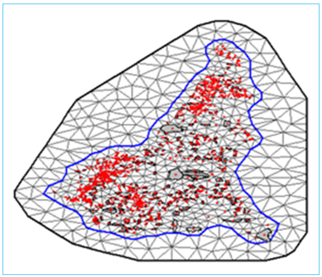
Figure 14.1: The Delaunay Triangulation of a Sample Mesh used for the INLA-SPDE implementation. The red points are the centroids of the spatial units.
14.4 Posterior Simulation and grid cell prediction
Usually, within the context of population estimation, interest is not only on the point estimates or the high resolution gridded population estimates at pixel and administrative levels, but also on the uncertainties around the estimates which are key to humanitarian intervention purposes. R-INLA only automatically calculates the 95% credible intervals for the mean values as part of the model outputs with no inbuilt functionality for calculating the quantiles of totals because the sum of quantiles is not the same as the quantile of totals. One solution to this challenge is to draw samples from the (approximate) joint posterior distribution of the latent field and hyperparameters given the data \(\pi(w, \theta |y\) and then evaluate the desire summary statistics of interest from the respective sampling distributions (e.g Gómez-Rubio et al. 2021).
Besides, drawing samples from the conditional distribution of a given parameter \(θ_1\), say, and then averaging over all the iterations will normally improve the estimation of the posterior marginal distribution \(π(θ_1│θ_2,y)\). This may be viewed as synonymous to the Rao-Blackwellization theory since group averaged estimators cannot increase the variance (Blackwell 1947, Rao 1992, Robert & Roberts 2021)
Thus, to obtain improved estimates of population with lower variance as well as the grid cell level administrative units level estimates along with the corresponding uncertainties, we can carry out posterior simulation using the five (5) key steps outlined below.
Posterior Simulation Steps
Specify and fit the INLA model using the inla() function setting config = TRUE within the control.compute argument. This allows INLA to draw samples from the (approximate) joint posterior distribution\[ \pi(w̃, θ̃ | ỹ) \] obtained, when prompted.
Using the (approximate) joint posterior distribution obtained in step 1, draw \(N\) samples of the latent field \(\{w̃_t\}_{t=1}^T\) and hyperparameters \(\{\thetã_t\}_{t=1}^T\) via the
inla.posterior.sample()function of the R-INLA package. This entails refitting the INLA model \(N\) times while allowing some variabilities within the random parameters. Note that the number of iterations \(T\) is variable, and the larger the better. However, computational cost would also increase with \(T\).For the \(G\) 100m × 100m square grid cells, define a \(G \times D\) projection matrix \(\tilde{A}_{gd}\) to project the grid cell level values at the mesh nodes.
For \(t\) in 1 to \(T\), do the following:
Select the \(t\)-th sample from the joint posterior \(\{w̃_t, θ̃_t\}\).
Using the scaled grid cell values of the covariates used in the model fitting stage at step 1, along with the intercept and the associated fixed effects coefficients \(\beta = (\hat{\beta}_0, \hat{\beta}_1, \ldots, \hat{\beta}_8)\), and the estimates of the random effects therein, predict the population density \(\hat{D}_{g,t}\) for each pixel based on (8.10). The random effects values are simulated from their respective posterior means, that is,
\[\begin{equation} \gamma_{gt} \sim \text{Normal}(0, \sigma_\gamma) \tag{14.1} \end{equation}\]
where \(\gamma \in \{f_p, f_r, \varepsilon\}\) and \(\sigma_\gamma > 0\) is the estimated variance for each random effect obtained in step 1.
- Using the predicted density and the observed building counts within a given grid cell, obtain the predicted population counts as
\[\begin{equation} \hat{y}_{g,t} = \hat{D}_{g,t} \times B_g \tag{14.2} \end{equation}\]
Repeat sub-steps (a) to (c) until a sample of the desired size is obtained.
Store the predicted population density and population count across the grid cells.
- From the stored simulated posterior samples, generate the various summary statistics such as:
- Mean grid cell level population density is obtained as the average predicted population densities across the entire sample of size T for the g-th grid cell.
\[\begin{equation} \overline{D}_g = \frac{1}{T} \sum_{t=1}^T \hat{D}_{g,t} \tag{14.3} \end{equation}\]
Mean grid cell population count is obtained as the average predicted population count across the entire sample of size \(T\) for the \(g\)-th grid cell. \[\begin{equation} \overline{y}_g = \frac{1}{T} \sum_{t=1}^T \hat{y}_{g,t} \tag{14.4} \end{equation}\]
Grid cell level uncertainties in the estimates of the grid cell population density and population count are based on the 95% credible interval obtained by taking the 2.5% and 97.5% quantiles of the \(g\)-th grid cell samples \(\hat{y}_{g,1}, \hat{y}_{g,2}, \dots, \hat{y}_{g,T}\) and \(\hat{D}_{g,1}, \hat{D}_{g,2}, \dots, \hat{D}_{g,T}\) for population count and population density, respectively. Alternatively, the pixel level upper and lower bounds estimates of uncertainties can be obtained as confidence intervals using for example, the lower bound can be calculated as
\[\begin{equation} \text{lower}^{(g)} = \overline{w}_g - 2\sigma_g \tag{14.5} \end{equation}\]
while the upper bound is given by
\[\begin{equation} \text{upper}^{(g)} = \overline{w}_g + 2\sigma_g \tag{14.6} \end{equation}\]
where the grid cell level standard deviation, \(\sigma_g\), is given by
\[\begin{equation} \sigma_g = \sqrt{\frac{1}{T-1} \sum_{t=1}^T (\hat{y}_{g,t} - \overline{w}_g)^2} \tag{14.7} \end{equation}\]
and \(\overline{w}_g \in \{\overline{D}_g, \overline{y}_g\}\).
The lower and upper bounds of the estimates provide an indication of the variability around the posterior estimates. A unique measure of \(uncertainty^{(g)}\) may then be derived as the average deviation given by \[\begin{equation} \text{uncertainty}^{(g)} = \frac{\text{upper}^{(g)} - \text{lower}^{(g)}}{\overline{w}_g} \tag{14.8} \end{equation}\]
- Obtain a distribution of the population totals at the various administrative levels: For each iteration, obtain the total population \(\hat{y}_t\) by summing the predicted count over all the grid cells, that is, \[\begin{equation} \hat{y}_t = \sum_{g=1}^G \hat{y}_{g,t} \tag{14.9} \end{equation}\]
Thus, the administrative level summary statistics of interest will then be obtained from the distribution of the total counts for all the \(T\) iterations \(\hat{y}_1, \hat{y}_2, \dots, \hat{y}_T\), so that the mean total count within a given administrative unit \(\overline{y}_{\text{admin}}\) is given by \[\begin{equation} \overline{y}_{\text{admin}} = \frac{1}{T} \sum_{t=1}^T \hat{y}^{(t)} \tag{14.10} \end{equation}\]
The standard deviation \(\sigma_{\text{admin}}\) is given by \[\begin{equation} \sigma_{\text{admin}} = \sqrt{\frac{1}{T-1} \sum_{i=1}^T (\hat{y}_t - \overline{y}_{\text{admin}})^2} \tag{14.11} \end{equation}\]
Similarly, the measures of uncertainty are then obtained as the 95% credible intervals using the quantile() function of base R set at 2.5% for the lower bound and at 97.5% for the upper bound. The uncertainty can also be given as confidence intervals using,
\[\begin{equation} \text{lower} = \overline{y}_{\text{admin}} - 2\sigma_{\text{admin}} \tag{14.12} \end{equation}\]
while the upper bound is given by \[\begin{equation} \text{upper} = \overline{y}_{\text{admin}} + 2\sigma_{\text{admin}} \tag{14.13} \end{equation}\]
In addition, a unique measure of uncertainty may be obtained for the lower administrative units as \[\begin{equation} \text{uncertainty} = \frac{\text{upper} - \text{lower}}{\overline{y}_{\text{admin}}} \tag{14.14} \end{equation}\]
Similar to the usual posterior sampling using methods such as MCMC, one may wish to view the mixing and distribution of the posterior samples across the parameter space using trace plots and histograms. However, unlike in the MCMC where these graphs are used to check convergence of the Markov chains, here the graphs are for descriptive statistics because the samples are drawn from the ‘true’ joint posterior density. The final estimates produced from the posterior simulations can be obtained in various formats as data tables, maps or raster files.
14.5 Model Fit Checks and Cross-Validation
A number of model fit checks and cross validations can be conducted to assess the goodness-of-fit and the predictive ability of models. These metrics include the the Widely Applicable Information Criterion (WAIC, Watanabe 2013), the Deviance Information Criterion (DIC, Spiegelhalter et al. 2002), and Conditional Predictive Ordinate (CPO, Pettit 1990). While the WAIC which is similar to the DIC measures the goodness-of-fit of a model based on model complexity with a smaller value indicating a better fit, the CPO is a cross-validatory criterion which calculates the probability of observing a held-out observation not used in model training. In addition, further predictive ability of the best fit model can also assessed based on k-fold cross validation technique in which the dataset is divided into two parts such that the model is trained with 80% of the data and then used to predict the 20% of the test samples that were held out. The process is then repeated k times with different samples making up the 20% test sample. We can also use other model fit metrics such as the Mean Absolute Error (MAE), Root Mean Square Error (RMSE), Pearson Correlation between the predicted and the observed values and the proprtions of observations that are within the 95% credible interval of the predictions to assess our model goodness-0f-fit and the predictive ability of models.
Mean Absolute Error (MAE) provides a measure of the average magnitude of errors within a set of predictions irrespective of the direction. It is calculated using
\[\begin{equation} \text{MAE} = \frac{1}{N} \sum_{i=1}^N |y_i - \hat{y}_i| \tag{14.15} \end{equation}\] where, \(y_i\) and \(\hat{y}_i\) are the observed and predicted values, respectively. The model with the smaller MAE value provides a better fit.
Root Mean Square Error (RMSE) is similar to the MAE in that they both provide an idea on the average magnitude of prediction error. However, the RMSE is found to be more useful when large errors are not desirable. RMSE is given by
\[\begin{equation} \text{RMSE} = \sqrt{\frac{1}{N} \sum_{i=1}^N (y_i - \hat{y}_i)^2} \tag{14.16} \end{equation}\]
Similar to the MAE, models with lower RMSE values provide better fit.
Proportion of the observations that are within the 95% credible interval of the predictions: The INLA-SPDE estimates include estimates of the uncertainties along with the mean values. One way of assessing these measures of uncertainties across the various models is to calculate the proportion of the observations that are within the 95% credible interval of the predictions.
\[\begin{equation} \text{INCI} = \frac{1}{N} \sum_i I(y_i) \tag{14.17} \end{equation}\]
where \(I(y_i)\) is an indicator function defined as \[I(y_i) = \begin{cases} 1, & \text{lower} \leq y_i \leq \text{upper} \\ 0, & \text{Otherwise} \end{cases} )\] where lower and upper are the 2.5% and 97.5% quantiles of the predicted values, respectively.
Pearson correlation between the predicted test values and the observed values: Another key model validation metric utilised for the cross-validated predictions is the (pearson) correlation coefficient \(r: -1 \leq r \leq 1\) between the values predicted for the withheld data and the actual observations withheld. This gives an indication of how strongly or how weakly the predicted values are in agreement with the observed values with values closer to 1 and -1 indicating high positive and high negative relationships, respectively. This is obtained using the equation
\[\begin{equation} r = \frac{\sum_i (y_i - \overline{y})(y_i^{(\text{pred})} - \overline{y}^{(\text{pred})})}{\sqrt{\sum_i (y_i - \overline{y})^2 \sum_i (y_i^{(\text{pred})} - \overline{y}^{(\text{pred})})^2}} \tag{14.18} \end{equation}\]
where \(y_i, \overline{y}, y_i^{(\text{pred})}\) and \(\overline{y}^{(\text{pred})}\) are the observed values, mean of the observed values, the predicted values, and the mean of the predicted values, respectively. Note that Equation (14.18) can be simply written as
\[\begin{equation} r = \frac{\text{Cov}(Y, Y^{(\text{pred})})}{\sigma_Y \sigma_{Y^{(\text{pred})}}} \tag{14.19} \end{equation}\]
where, \(\text{Cov}(Y, Y^{(\text{pred})})\) is the covariance between the observed \(y\) and the predicted value \(y^{(\text{pred})}\), and \(\sigma_z, z \in \{y, y^{(\text{pred})}\}\), are the corresponding standard deviations.
14.6 Contribution
This chapter was written by Chris Nnanatu