18 South Sudan (v2)
South Sudan 2020 gridded population estimates from census projections adjusted for displacement, version 2.0
18.1 Introduction
South Sudan’s last population and housing census was conducted in 2008 prior to its independence from Sudan in 2011. Estimating the population of South Sudan and mapping its spatial distribution is incredibly challenging due to ongoing conflict, flooding and famine that continues to drive large scale movement within the country as well as across national borders into neighbouring countries. This chapter presents an approach that integrates several different data sources available at differing spatial scales to estimate South Sudan’s population at a high spatial resolution in 2020. This chapter describes the methods used to produce the South Sudan 2020 gridded population estimates from census projections adjusted for displacement, version 2.0 (Dooley et al. 2021). This approach models the population distribution to likely settled locations and adjusts for displacement. Conceptually, the population in a given location is expected to follow:
The key elements of this approach are:
- disaggregating projected census population estimates for 2020 to a high spatial resolution using a number of ancillary geospatial datasets, including building footprints, which depict factors known to relate to human population presence (baseline population)
- using geocoded internally displaced populations and building footprints to demarcate destination spatial extents of displaced populations (in-displacement)
- modelling where people have been displaced from at a high spatial resolution using geospatial data including conflict locations (out-displacement)
- combining the projected population estimates (in a) and displaced population estimates (in b and c) to produce the final adjusted population estimates that account for displacement (final population) This chapter present model assessments, provide example areas from the results and discuss future work needed to improve mapping efforts in South Sudan. Note that the final dataset is most likely to represent South Sudan’s population distribution as of September 2020 given the age of the input data.
18.2 Methods
All data preparation and analysis was carried out using R version 4.0.2 (R Core Team 2020b). We used the World Geodetic System 1984 (WGS84) projection system for all geospatial data. If input data was not in this projection, the data was converted accordingly. We used the WorldPop South Sudan mastergrid for the grid positioning of all rasters throughout the analysis. All output data is provided in raster format with WGS84 projection and approximately 100m x 100m resolution (0.0008333 decimal degrees grid).
18.2.1 Boundaries, settled area and unadjusted (baseline) county population totals
To define our study area, we used the United Nations Office for the Coordination of Humanitarian Affairs (OCHA) operational administrative level 2 boundaries (counties) dataset OCHA. Grid cells within this area were defined as ‘settled’ if they contained any building centroids in the Digitise Africa building footprints dataset (Ecopia.AI & Maxar Technologies 2020c) for South Sudan and its neighbouring countries (Central African Republic, Democratic Republic of Congo, Ethiopia, Kenya, Sudan, Uganda). For the unadjusted (baseline) population estimates, we used county level population projections for 2020 from the 2008 census produced by the South Sudan National Bureau of Statistics (National Bureau of Statistics, 2015). These projections are derived using fertility and mortality rates, and do not account for displacement.
18.2.2 Mapping of internally displaced persons
The International Organisation for Migration IOM collect extensive information on internally displaced persons (IDPs) in South Sudan. From 1st July 2020 to 30th September 2020, IOM conducted Round 9 of their ‘Baseline Assessment’ of IDPs Displacement Tracking Matrix which includes estimated numbers of IDPs at more than 2,000 locations across South Sudan. The data is collected from key informants at each location and verified by the IOM team who report on the consistency of the data and whether it is in line with observations. IOM’s Baseline Assessment Round 9 covers almost every area of the country and provides the highest resolution of locations of IDP populations compared to other datasets where estimates are given for large areas only. However, we acknowledge that there is likely to be large and varying uncertainty in the IDP counts. In this study we do not consider the uncertainty in IDP estimates as it would be incredibly difficult to quantify given the data collection methodology. All IOM data mentioned in this report refers to their Baseline Assessment Round 9. Note that we refer to a single location of IDPs as an IDP population.
As of September 2020, IOM reported 1,615,765 IDPs residing inside South Sudan. Of the total number of IDPs, an estimated 554,081 people were displaced from a different county and 1,061,684 people were displaced from within their same county. All reported IDP populations were 28,000 people or less, with the exception of UNMISS Bentiu Protection of Civilians camp which had 97,321 IDPs.
In this study we aim to identify the likely area in which IDP populations may be living, which then allows us to redistribute those populations over the most likely settled areas. This is necessary because defined boundaries of the areas in which IDPs reside are not available. IOM classifies locations of IDP populations as either a ‘displacement site’ or within a ‘host community’. We assume that ‘displacement sites’ have been purposefully constructed or converted to accommodate IDPs and, therefore, are occupied by IDPs only. ‘Displacement sites’ include UN Protection of Civilians sites and converted public buildings such as schools. Conversely, we assume that host communities can have both IDPs and non-IDPs. Because of these assumptions, we mapped the area occupied by ‘displacement sites’ first and then excluded these areas for the mapping of all other populations (IDP host communities, unadjusted (baseline) population and areas people have been displaced from).
There were a total of 99 open ‘displacements sites’ recorded by IOM (a further 23 closed sites were also reported to have no IDPs present as of September 2020). There was one open site recorded for Korijo IDP Camp Zone 1, 2 and 3, and we split this into three separate sites based on the proportion of IDPs across the three camps and their locations in July 2017 (IOM 2017). We merged the sites recorded for ‘Panyiduay Hospital’ and ‘School Panyiduay’ as they had the same location coordinates. This meant that IDPs across the two sites occupy the same location in our final dataset.
After these data edits, we mapped the resulting 100 ‘displacement sites’ by identifying the nearest settled grid cell to the site’s recorded location coordinates and then buffering an area around the focal cell. The size of the buffered area varied per site and was big enough such that the number of IDPs per settled cell did not exceed 500 people. We capped the buffer size to a maximum of 3.5km, and therefore allowed more than 500 people per settled cell where the maximum buffer was reached. The distance restriction was implemented so that ‘displacement sites’ weren’t incorrectly mapped as sparse and sprawling. We used a people per cell restriction rather than people per building. This is because ‘displacement sites’ are likely to have non-permanent structures such as tents and so we didn’t want to rely on the count of building footprints in these areas reflecting the situation at the time of data collection. The high maximum value of 500 people per grid cell was selected to allow for potentially high population densities in low resource situations and to restrict the spatial areas covered by these IDP only sites to realistic spaces in urban areas.
We cross referenced a subset of the resulting ‘displacement sites’ areas with publicly available spatial data relating to 22 UN IDP camps UN IDP Camps and found that the areas matched well. However, there is no available spatial data for non-UN camps and cross referencing was therefore not possible for non-UN ‘displacement sites’. In the absence of this data, we highlight that there are potential uncertainties in our results. In particular, the maximum of 500 people per grid cell may have been too high for rural ‘displacement sites’ and may have led to spatial extents that are too small (for example, if the maximum was 250, the spatial extent would have been bigger because the buffer size would have needed to be bigger to allow for lower people per cell). With limited data available for non-UN sites, it is outside the scope of this study to assess our mapped ‘displacement sites’ thoroughly, and we recommend that further evaluation be done in collaboration with NBS, IOM and other data collectors.
There were 2,097 ‘host community’ sites with recorded IDPs. To map the spatial extents of these populations from their georeferenced point locations, we incrementally increased a buffer around the location until there was no more than 1 IDP per building within the buffer. Given the possible national population totals, reasonable household sizes of 5.5-6.5 persons (average household size in the 2008 census was 5.9) (Minnesota Population Center 2020) and the number of building footprints, we estimate that approximately 50% of the building footprints are residential. Based on this assumption, along with a reasonable average limit of 2 IDPs per residential building in host community settings, we considered 1 IDP per building to be a sensible maximum, while acknowledging that this could vary significantly between IDP populations across the country. If buffer areas of different IDP populations overlapped, we allowed the limit per building within the overlapping area to increase (with the limit being 1 IDP per building per IDP population). We applied a maximum buffer of 50km in order to prevent IDPs being mapped in potentially incorrect locations. We chose 50km because there was always at least one building within that distance of the recorded IDP point location.
18.2.3 Mapping of unadjusted population (population distribution in the absence of displacement)
We disaggregated the 2020 county level population projection estimates (National Bureau of Statistics 2015) to a high spatial resolution grid using a random forest machine learning-based dasymetric approach (Stevens et al. 2015d). This approach allowed us to predict grid cell level population estimates based on modelled relationships with geospatial data (covariates) while preserving the projected county-level population totals. Here we used a bespoke set of covariates that included data potentially important for predicting the distribution of South Sudan’s unadjusted population projection. We started with a total of 36 covariates relating to land use types, physical attributes, climate and the built environment. The steps taken in our approach were:
- Prepare covariate layers so that their spatial extent matches the OCHA boundaries
- Mask out the areas considered to be IDP ‘displacement sites’ (e.g. UN Protection of Civilians sites, i.e. not ‘host communities’) across all covariates
- Calculate mean covariate values across the settled grid cells per county
- Calculate population density per county (population per settled area defined as the sum of areas of grid cell containing building centroids)
- Run iterations of the random forest model, with log mean population density as the response variable, dropping covariates that have low importance scores in each
- Run the final model that included important covariates only
- Predict log population density weighting layer using the final model and covariate values for each settled grid cell (excluding those classified as a displacement site)
- Distribute the aggregate (county-level) population counts to grid cells using the weighting layer
18.2.4 Mapping locations where people have been displaced from
Data on where people have been displaced from is notoriously difficult to collect due to multiple settlement and administrative unit names used for given locations and challenges in recording multiple origins across large displaced populations. The IOM data summarises where the majority of current IDPs have been displaced from. This is reported for each IDP population (i.e. at each destination location) and by the following arrival time periods: a) 2014-2015; b) 2016-2017; c) 2018 pre- Revitalised Agreement for the Resolution of Conflict in South Sudan (R-ARCSS); d) 2018 post- R-ARCSS; e) 2019; and, f) 2020. While we know that different IDPs may have arrived at a destination location from different places of origin during a given time period, this data is the best resource compared to other available data. From this county origins data, we calculated the total estimated number of IDPs that had been displaced from each county. In addition to 1,615,765 IDPs, there was an estimated 2,185,117 refugees living outside of South Sudan (as of September 2020) (UNHCR 2020). Very little data exists for the place of origin of these refugees. Here we combined information from two datasets to estimate the number of refugees displaced from each county but emphasise the unquantified and potentially large uncertainty in these estimates.
The first dataset was a household survey conducted by the UN Refugee Agency (UNHCR) in each of the countries surrounding South Sudan (UNHCR 2019). This survey covered a total of 6,964 households across 15 refugee camps: Ethiopia (3 camps), Uganda (3 camps), Sudan (2 camps), Kenya (3 camps), the Democratic Republic of Congo (3 camps) and the Central African Republic (1 camps). While data on county of origin was not available, the survey reported the proportion of respondents from each state in South Sudan. We applied these proportions to the total number of refugees to estimate the numbers displaced from each state, and then split these state level estimates across counties based on the reported ‘not yet returned’ estimates provided at each location surveyed in the IOM Baseline Assessment. ‘Not yet returned’ is an estimate of how many people have been displaced from the survey location and not returned, reported by the key informants. The ‘not yet returned’ numbers have a very large level of uncertainty due to recall biases and gaps in coverage for areas with consistently high conflict (as the Baseline Assessment targets locations of displaced persons and/or returnees, not areas where there are neither). Therefore, we did not use the exact numbers but instead used the proportion of ‘not yet returned’ across counties within a given state. The ‘not yet returned’ estimates were used for this step in estimating the origin of refugees, rather than using the origin data of IDPs because the origins of those displaced internally to neighbouring counties can be very different to the origins of those displaced into neighbouring countries. For example, Yei county has experienced some of the highest levels of conflict in the country yet there are very few IDPs reportedly displaced from Yei. Instead, people were forcibly displaced into Uganda, and this is evident in the relatively high estimates of ‘not yet returned’ for the county.
After applying this procedure we found that four counties (Ibba, Western Equatoria; Morobo, Central Equatoria; Nagero, Western Equatoria; Panyikang, Upper Nile) had less than 10% of their census projection population remaining when the total number of people displaced from them was subtracted. Because of the high uncertainty in these displacement origin numbers, we re-estimated the total number of refugees from these four counties such that they did not exceed 90% of the census projection. In reality, it is possible that county populations are depleted to a larger extent, but we erred on the side of caution to avoid under-representing current populations of these counties in the final dataset. Reducing the number of refugees displaced from these four counties resulted in a total of 2,062,059 refugees being accounted for instead of the reported 2,185,117.
We summed the estimated number of IDPs and refugees displaced from each county, and then applied the random forest disaggregation methodology to map estimates of people displaced from each settled grid cell across the country. For this we used the same steps as outlined in Mapping of unadjusted population (population distribution in the absence of displacement). See Figure 18.5 for the distribution of estimated counts of people displaced from each county as well as the model response variable (log estimated density of people displaced from each county). Again, these settled grid cells did not include those classified as purposefully constructed or converted ‘displacement sites’. In addition to the 36 covariates used for predicting unadjusted population counts, we generated covariates relating to conflict as these are critical for predicting where people have been displaced from. We used the reported conflict events between January 2014 and September 2020 in the Armed Conflict Location Events Database (Raleigh et al. 2010). After initial comparisons of different potential measures, we created covariates for distance to: a) all ‘Battles’ and ‘Violence against civilians’ events; b) all events that resulted in 5 or more fatalities; c) all events that resulted in 20 or more fatalities; and, d) all events that resulted in 50 or more fatalities. Each layer was created separately for each year between 2014 and 2020.
18.2.5 Final population distribution accounting for displacement
To produce the final, high spatial resolution gridded population distribution, we simply applied the following equation using the grid cell level datasets:
18.3 Results
18.3.1 Mapping of internally displaced persons
The mean and median number of IDPs per grid cell was: 344 and 224 for ‘displacements sites’ and 4 and 2 for ‘host community’ sites (Figure 18.1). Our method of incrementally increasing the buffer around georeferenced locations was able to capture a reasonable area of buildings that could house IDPs in urban and many rural areas. Figure 18.2 shows an example of the areas mapped as IDP locations across South Sudan’s capital, Juba. In some sparse rural areas, particularly Jonglei in the east of the country, IDP coordinate locations were very far away from their nearest building footprints. Further work is needed to understand the overlap of point locations and building footprints in the context of individual IDP population, e.g. what type of community do the IDPs join? What is the primary housing type? Is the spatial extent in which IDPs live fluctuating significantly in short periods of time? With limited data available on the spatial extent of non-UN camps, it is outside the scope of this study to address these questions and thoroughly evaluate the mapped IDPs. Here we provide a starting point to facilitate future work on mapping IDPs from community level point locations, and recommend further evaluation in collaboration with NBS, IOM and other data collectors.
A total of 1,431 grid cells out of 1,054,006 settled grid cells were classified as ‘displacement sites’ across the country. These cells were considered to contain IDPs only and were not included in the mapping of the unadjusted census projections and where people have been displaced from.
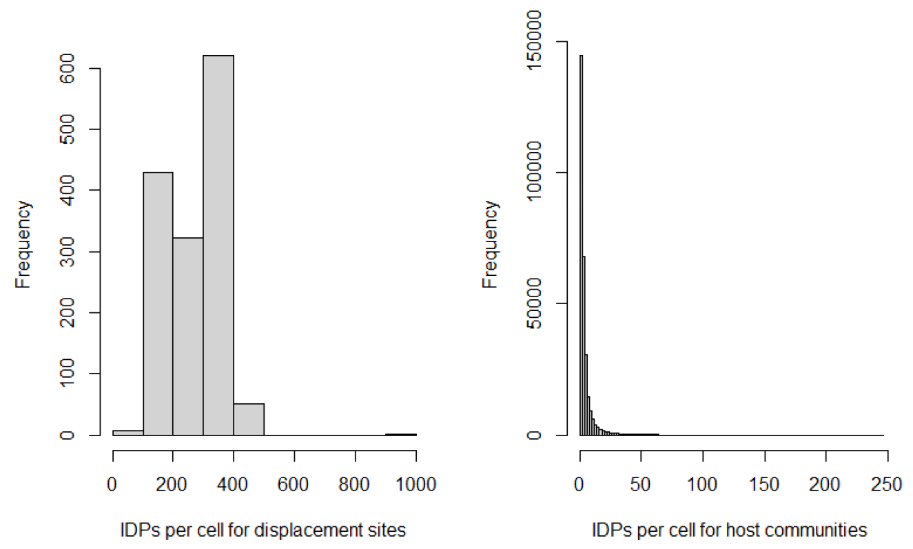
Figure 18.1: Histograms of IDPs per cell for ‘displacement sites’ (left) and ‘host communities’ (right).
![Mapped spatial extents of IDP populations across Juba derived using reported point locations and estimates IDP counts as of September 2020 [@IOM_SSD2] and building footprint [@EcopiaAI_SSD].](pic/SSD_displacement.png)
Figure 18.2: Mapped spatial extents of IDP populations across Juba derived using reported point locations and estimates IDP counts as of September 2020 (IOM 2021) and building footprint (Ecopia.AI & Maxar Technologies 2020c).
18.3.2 Mapping of unadjusted population (population distribution in the absence of displacement)
The variance explained was 50.02% and the mean of squared residuals was 0.28, for the final random forest model used to predict the unadjusted census population counts at a high spatial resolution. Given the relatively low number of administrative unit (79 counties) to fit the model and the high uncertainties in projections from a census conducted 12 years ago, we consider these results to be reasonable. Figure 18.3 shows covariate importance for the final model and highlights that specific monthly precipitation means and building footprint metrics were among the best variables from the covariate set for estimating the spatial distribution of the unadjusted population.
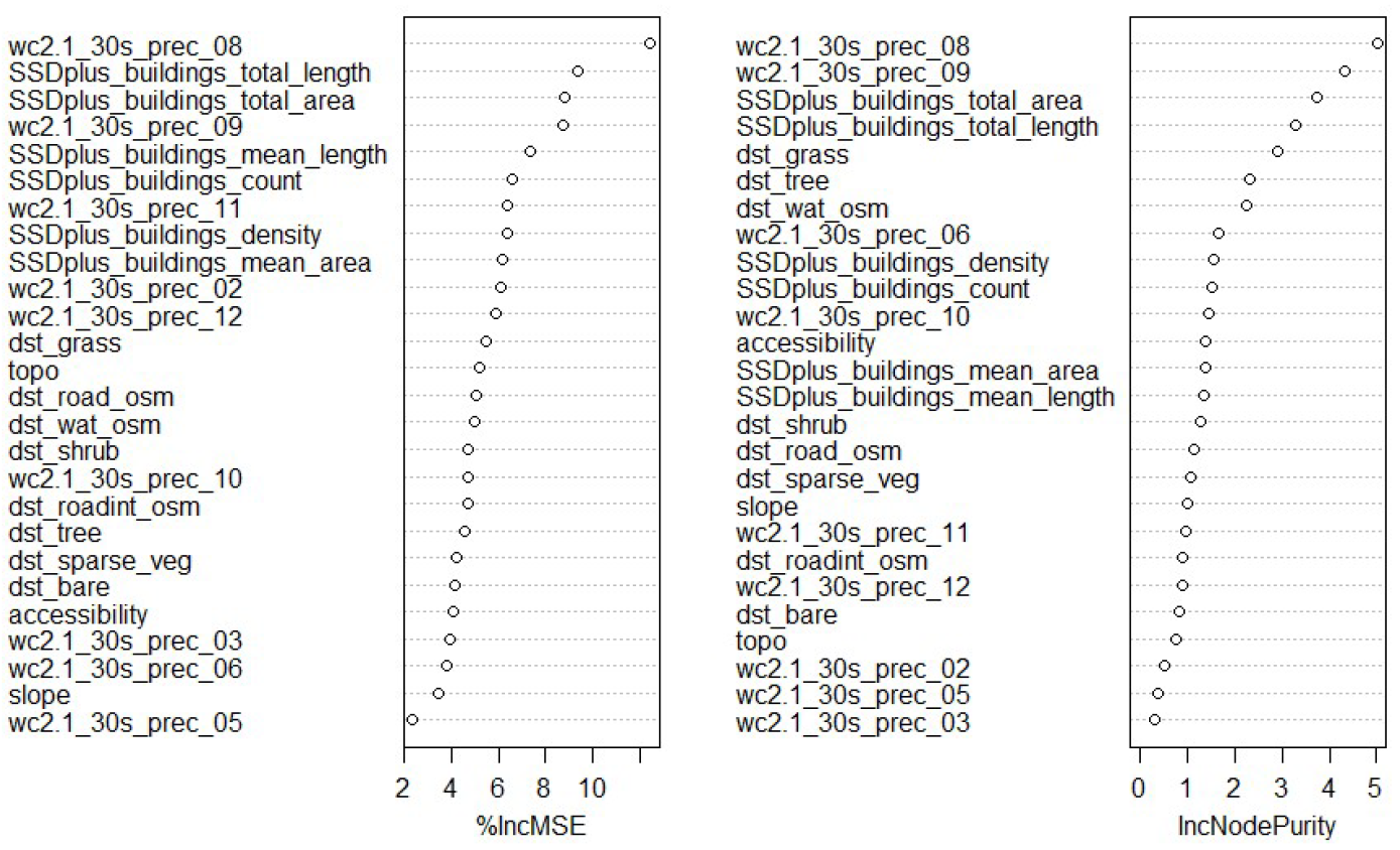
Figure 18.3: List of covariates used to predict the unadjusted census population counts, ordered by importance in the model. The %IncMSE indicates the increase of the mean squared error and the IncNodePurity is a measure of the total increase in node purity, when the given variable is randomly permuted.
18.3.3 Mapping of where people have been displaced from
For the final random forest model estimating the origin of displacement, the variance explained was 46.34% and the mean of squared residuals was 0.81. We found that the conflict covariates were the most important of the covariates set (Figure 18.4). These results show that there is huge potential for using geospatial layers derived from conflict data to map and understand where people have been displaced from. Again, the level of variance explained by the model is reasonable given that the model is based on only 79 administrative units and the high uncertainties in county level counts. The county level estimates were based on summaries of place of origin for whole IDP populations as well as very limited origin data for refugees. In order to improve the accuracy of mapping where people have been displaced from, finer scale origin data is needed
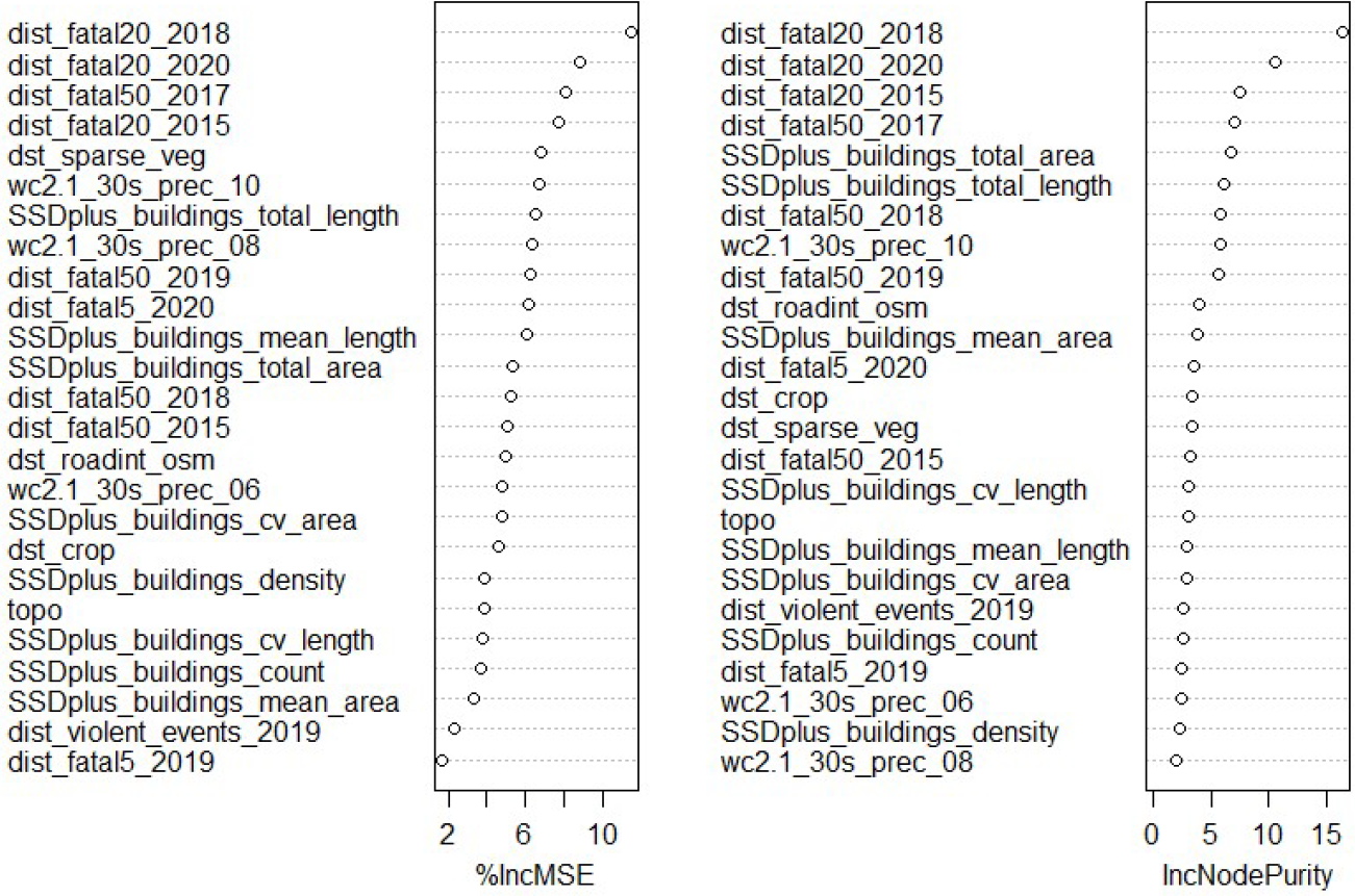
Figure 18.4: List of covariates used to predict the locations where people have been displaced from, ordered by importance in the model. The %IncMSE indicates the increase of the mean squared error and the IncNodePurity is a measure of the total increase in node purity, when the given variable is randomly permuted.
In a small proportion of grid cells (12,638 out of 1,054,006) we found that the estimated number of people displaced from them was larger than their unadjusted population count. This was not unexpected given the high levels of uncertainty in both the census projections and the counts of people displaced from counties. This shows that the county level uncertainty propagated to the grid cell level. The affected grid cells were concentrated to a small number of counties in Upper Nile State and along the southern national border, and correspond to the areas of highest conflict (see top-right map of Figure 18.5 for variation in estimates of people displaced across counties with lighter colours indicating counties where large numbers have been displaced from). For these grid cells where the estimated number of people displaced from them exceeded their unadjusted population count, we replaced the value in the origin of displacement layer with the unadjusted population count, such that the final population estimates are set to zero.
![Distribution of county level counts in absolute numbers (top plots) and log densities (bottom plots). In this study we used the United Nations Office for the Coordination of Humanitarian Affairs (OCHA) operational administrative level 2 boundaries (counties) dataset [@OCHA], as shown here.](pic/SSD_response.png)
Figure 18.5: Distribution of county level counts in absolute numbers (top plots) and log densities (bottom plots). In this study we used the United Nations Office for the Coordination of Humanitarian Affairs (OCHA) operational administrative level 2 boundaries (counties) dataset (United Nations Office for the Coordination of Humanitarian Affairs 2019), as shown here.
18.3.4 Final population distribution accounting for displacement
For the final population data, the mean, median and maximum grid cell level population counts were 10.6, 7.1 and 921.0 respectively. In Figure 18.6 we show the final state level totals and in Figure 18.7 we present the final population distribution across Juba.
![2020 state level population counts from census projections (unadjusted to account for displacement) and counts for the South Sudan V2.0 dataset that are adjusted to account for displacement. This is the number of refugees we deducted from the census counts given the available county level population data and place of origin information. The official number of refugees as of October 2021 was 2,185,117 [@UNHCR_2020].](pic/SSD_table.png)
Figure 18.6: 2020 state level population counts from census projections (unadjusted to account for displacement) and counts for the South Sudan V2.0 dataset that are adjusted to account for displacement. This is the number of refugees we deducted from the census counts given the available county level population data and place of origin information. The official number of refugees as of October 2021 was 2,185,117 (UNHCR 2020).
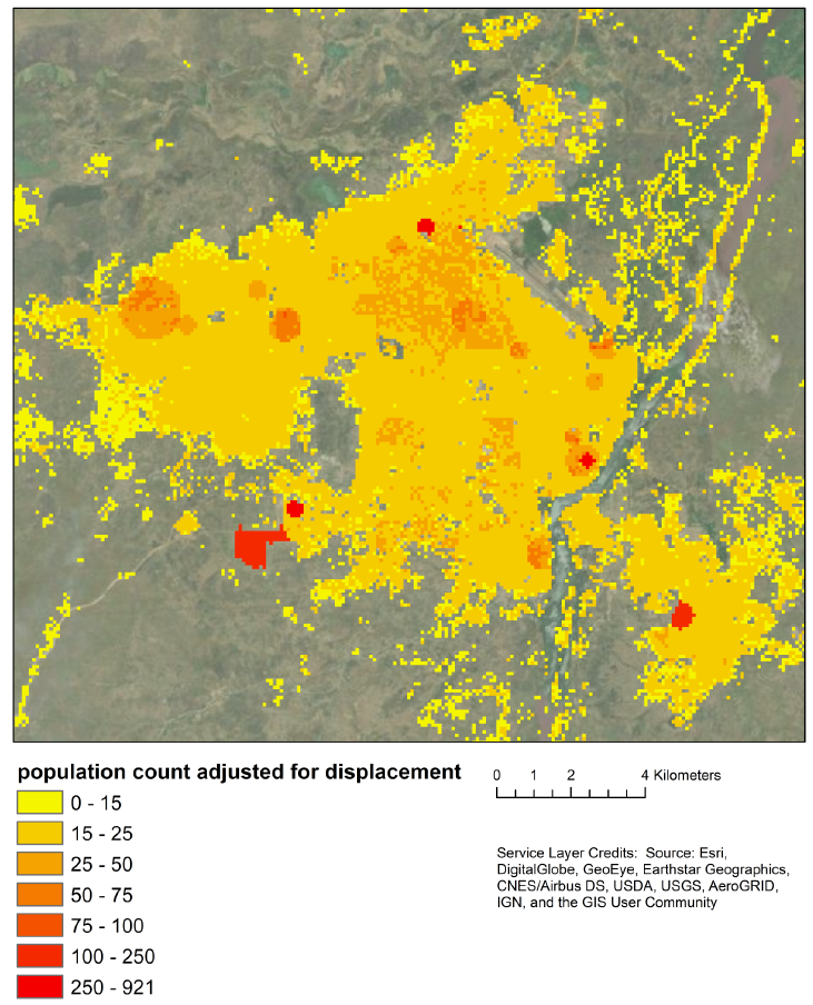
Figure 18.7: Final grid cell level population counts accounting for displacement across Juba. The highest population counts (red) can been seen in areas where ‘displacement sites’ are located and relatively high population counts (dark orange) in areas where IDPs are present in host communities.
18.4 Discussion
Here we present a unique approach for integrating different datasets to produce high spatial resolution population estimates that account for displacement in a high conflict and data limited setting. We estimate the approximate time point that the data represents as being September 2020, given the mix of input data. We recommend the following areas for future work:
Validation of IDP population spatial extents - here we applied a set of rules to map IDP populations, but further information about the populations is needed to help understand their densities compared to that of host populations.
Collating information on place of origin of displaced persons - there is very little coherent and accurate origin data. The UNHCR survey used in this study had a relatively small sample size and only reported data at the state level. Similar representative household surveys of displaced populations could provide valuable data on place of origin at a fine scale. This would open up options to carry out causal analyses as well as improve the county level estimates for the top-down approach we implemented.
Consideration of seasonal dynamics including nomadic groups.
Development of informative covariates for improving the accuracy of top-down models - uncertainty in county level counts needs to be reduced before this step, however, with more accurate estimates further testing of potential covariates could improve the results. Specifically:
– Additional covariates relating to fatalities and event types that could be derived from the conflict location data
– Alternatives to the flow accumulation covariate that may be indicative of flooding events, e.g. topographic wetness index. Although natural disasters were responsible for only < 3% of IDP displacement (IOM 2017, 2021)
– Additional climatic variables - here we only used monthly precipitation. We did test alternative models that included 3 month means and sums in place of the individual monthly precipitation covariates, but the latter produced better model fit. WorldClim provides other variables on temperature and additional metrics such as maximum and minimums.
Note: The gridded population estimates for SSD are available from the WorldPop Open Population Repository WOPR, and they can be visualized using the WOPR Vision web application (select “SSD v2.0”)
Contribution
This chapter and its corresponding dataset was led by Claire Dooley. Chris Jochem, Alessandro Sorichetta and Andy Tatem contributed to methods development. Oversight of the work was provided by by Attila N. Lazar and Andy Tatem