10 Ghana (v2)
A Bayesian approach to produce 100 m gridded population estimates using census microdata and recent building footprints
10.1 Introduction
Gridded population estimates can provide an important resource for planning government services, housing and population censuses, health and education initiatives, household surveys and other programmes in situations when there are no recent census data available. Gridded population estimates can be aggregated to estimate total populations for custom areas suited to individual project goals. WorldPop uses two general approaches for producing gridded population estimates: bottom-up and top-down (Wardrop et al. 2018a).
Top-down methods (Stevens et al. 2015a) disaggregate known population totals for administrative units into gridded population estimates at higher spatial resolution (e.g. 100 m). This approach is best for situations where reliable population totals for administrative units are available from a recent census or census projections. The population totals are disaggregated based on relationships with gridded geospatial covariates that are mapped consistently across an entire study area or region of interest such as nighttime lights, impervious surfaces, and distance to city centers. Top-down approaches are not reliable when population totals from a recent census are not available and population projections are not reliable due to population displacement, time since the last census, or other reasons.
Bottom-up methods (Leasure et al. 2020d) use population counts from a sample of locations (e.g. from household surveys) to produce gridded population estimates with full national coverage. This approach is best for situations when population totals from census are not available but recent household survey data are available with full enumeration of people in a sample of clearly defined survey locations. Like the top-down method, populations are estimated based on relationships with gridded geospatial covariates. Bottom-up methods are often based on Bayesian statistical models that provide robust estimates of uncertainty, whereas top-down models based on machine learning models (Stevens et al. 2015a) do not provide any confidence bounds on population estimates. One challenge with the bottom-up approach is that it requires geolocated household survey data that can be difficult to access due to privacy safeguards that must be put in place.
A method is needed that can produce robust gridded population estimates in situations where recent census data and geolocated household survey data are both unavailable. There are publicly available anonymized household survey data without specific location information that could be used for this purpose (e.g. IPUMS, DHS). The increasing availability of building footprints mapped from satellite imagery also provides a valuable source of information. A statistical method that measures statistical uncertainty for population estimates would be needed because the inherent uncertainty in population data that are not geolocated will likely produce population estimates with wide confidence intervals that would be important for end users to be aware of.
Our goal here was to develop a new Bayesian statistical model to estimate the number of households per building and people per household at sub-national spatial scales. We prioritized the use of publicly available data so that the method could be replicated across countries more easily. We demonstrated this new approach with a case study to produce gridded population estimates for Ghana. Our aim was to produce:
- 100-meter gridded population estimates with national coverage,
- Estimates of age-sex structure by region and settlement type,
- Estimates of people per household by geographic unit and settlement type,
- Estimates of households per building by geographic unit and settlement type, and
- Robust estimates of uncertainty for population estimates (and other parameters) at any spatial scale.
10.2 Methods
The total population for an area can be described as a function of the number of buildings:
\[ population = buildings \times \frac{households}{building} \times \frac{people}{household} \] We develop this equation into a hierarchical statistical model below, but first we will describe the sources of information needed to inform the parameters on the right side of the equation.
10.2.1 Data
Building footprints. We used rasterized counts of buildings within approximately 100 m grid cells across Ghana (Dooley et al. 2020a). These were derived from building footprints for sub-saharan Africa that were extracted from recent high-resolution satellite imagery (Ecopia.AI & Maxar Technologies, Inc. 2019-2021) (modal year = 2018, range = 2009 to 2019).
Census microdata. We used microdata samples from the 2010 Ghana census that were publicly available from IPUMS International (Minnesota Population Center 2019). This provides a count of the number of people from thousands of housing units with representative national coverage. Each household record is geo-tagged to geographic areas nested within larger regions. These level 1 and level 2 geographic boundaries (Fig. 10.1) were available for download from IPUMS International (Minnesota Population Center 2019).
There were no GPS coordinates associated with these household-level survey data for privacy reasons. The absence of specific location information is one of the primary challenges to overcome with the statistical model. Geospatial covariates that are usually fundamental for bottom-up statistical models (Wardrop et al. 2018a, Leasure et al. 2020d) cannot be used here because we do not know the exact locations of the household surveys.
We used this to estimate the average number of people per household within sub-national geographic units. We also used these data to estimate the demographic composition of the populations in these areas by age and sex. We will assume that these parameters have not changed since 2010 when the census was conducted.
Population totals. We used population totals for level 3 administrative units that were projected to the year 2018 from the last census (WorldPop & CIESIN 2018a). We also used the level 3 administrative boundaries used for those projections (WorldPop & CIESIN 2018b) (Fig. 10.1).
We used this to estimate the average number of housing units per building. We used projections to the year 2018 to match the year of the building footprints.
Settlement type. We used the urban and rural classifications of enumeration areas from the 2010 Ghana census (Ghana Statistical Services 2010). We summarized the original three settlement types into urban and rural classes based on guidance from Ghana Statistical Services. We assumed that this was the same urban and rural classification reported in the census microdata from IPUMS International (Minnesota Population Center 2019).
Maps of settlement types, administrative boundaries, and IPUMS geographic regions (Fig. 10.1) were rasterized to a 100 m mastergrid matching the building footprints rasters (Dooley et al. 2020a).
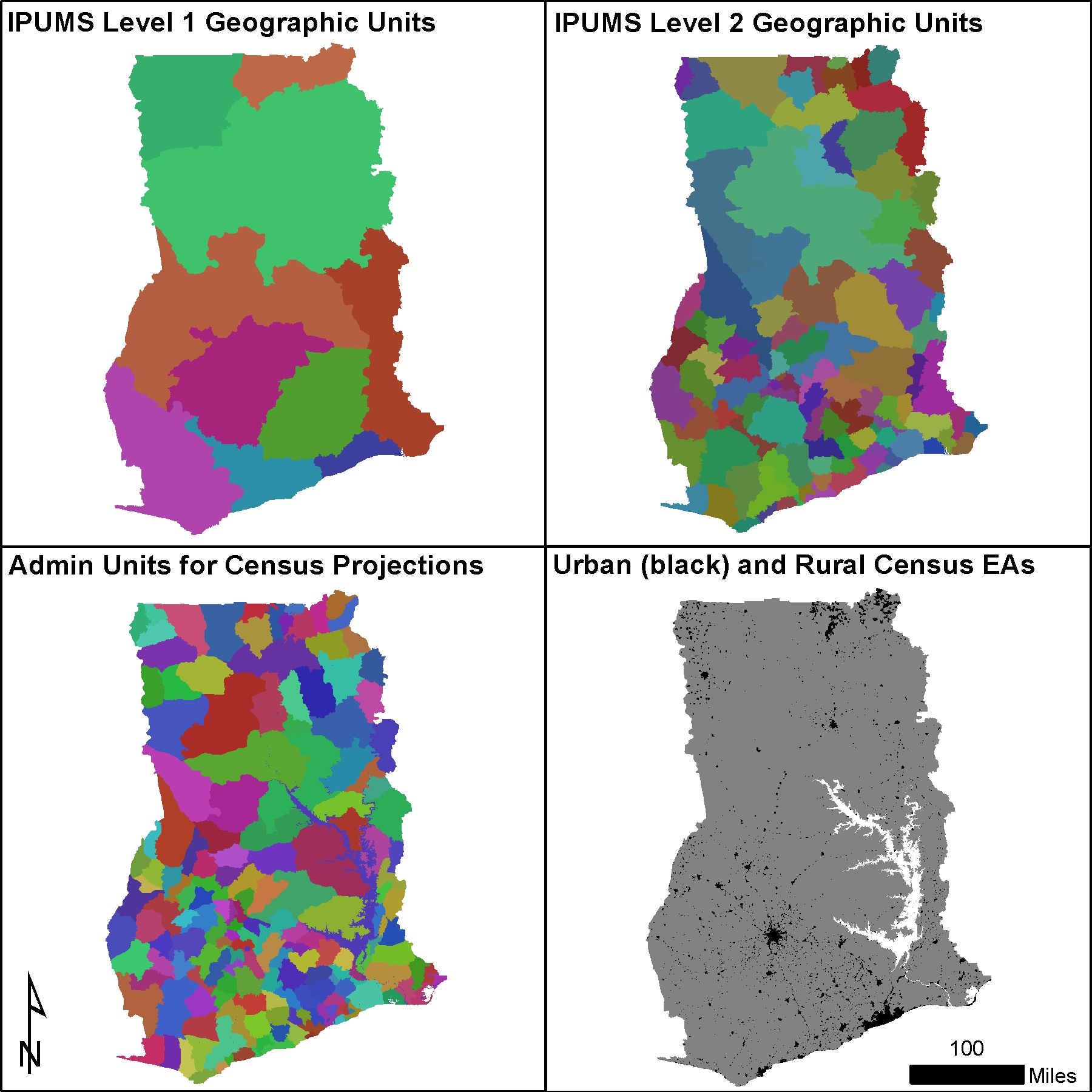
Figure 10.1: Geographic units used for modelling.
10.2.2 Statistical Model
We developed a Bayesian statistical model to estimate the average number of people per housing unit and the average number of housing units per building from these data.
Indexing
The indexing used throughout the model description (below) is as follows:
Households (h) contained within the IPUMS data. There was a total of 570,234 households from the Ghana census microdata and we used a representative 70% sample to fit our model (selected at random using the SAMPLE attribute of the IPUMS data). The remaining 30% was used for out-of-sample model validation.
Age-sex groups (k) that included 36 bins: under 1 year, 1 to 5 years, 80+ years, and 5-year intervals in between for both males and females.
Settlement type (t) for each enumeration area from the 2010 Ghana census. We summarized these as either urban (1) or rural (2).
Age-sex regions (r) were defined by the level 1 geographic boundaries from IPUMS (Minnesota Population Center 2019). We estimated the proportion of the population in each age-sex group for urban and rural areas within each of these 10 regions.
Household geographies (g) were defined by the level 2 geographic boundaries from IPUMS (Minnesota Population Center 2019). We estimated people per household for urban and rural areas within each of these 102 geographies.
Population units (u) were defined by the level 3 administrative boundaries from census projections (WorldPop & CIESIN 2018b). We estimated households per building for urban and rural areas within each of these 170 population units.
Locations (i) are 100-meter grid cells that were used for model predictions.
Population Estimates
To estimate the population for a given location \(i\), we used the following model:
\[\begin{equation} pop_i \sim \textsf{Poisson}(bldg_i \times hpb_{t_i,u_i} \times pph_{t_i, g_i}) \\ pop_{i,k} \sim \textsf{Multinomial}(pop_i, \theta_{t_i,r_i,k}) \tag{6.5} \end{equation}\]
\(pop_i\) is the total population estimated for location \(i\), and \(pop_{i,k}\) is the number of people within age-sex group \(k\). \(bldg_i\) is the observed number of building footprints at this location. \(hpb\) and \(pph\) are estimated parameters measuring households per building and people per household, respectively. In this portion of the model, the only observed data are the building counts \(bldg_i\), settlement type \(t_i\), and the three spatial unit IDs (\(g_i\), \(u_i\), and \(r_i\)). Note that we are assuming that the count of building footprints is equivalent to the true count of buildings.
Estimating the parameters \(hpb_{t,u}\), \(pph_{t,g}\), and \(\theta_{t,r,k}\) is the focus of the statistical model developed below.
People per Household (pph)
Single-person households are more common in the Ghana microdata than could be accounted for by a simple Poisson distribution to model household sizes, so we used a Hurdle model (Stan Development Team 2019a) to account for the one-inflated distribution. This involves two processes:
\(\alpha_{t,g}\) the probability that a household has only a single-person , and
\(\lambda_{t,g}\) the number of additional people in multi-person households other than the head of household.
These two parameters are the basis for estimating people per household \(pph_{t,g}\) by type and household geographic unit. The Ghana census microdata (IPUMS 2020) provided the data that we needed to fit this part of the model. This included a count of people and their ages from a representative sample of households across the country.
We used a beta-binomial model to estimate the probability of a single-person household \(\alpha_{t,g}\) in urban and rural settlement types \(t\) in each geographic area \(g\):
\[\begin{equation} single_{t,g} \sim \textsf{Binomial}(hh_{t,g}, \alpha_{t,g}) \\ \alpha_{t,g} \sim \textsf{Beta}(\frac{\bar{\alpha}_{t}}{\tilde{\alpha}}, \frac{1-\bar{\alpha}_{t}}{\tilde{\alpha}}) \tag{10.1} \end{equation}\]
where \(hh_{t,g}\) is the total number of households surveyed from settlement type \(t\) in geography \(g\), and \(single_{t,g}\) is the total number of single-person households surveyed. \(\alpha_{t,g}\) is the probability that a household contains only a single person. \(\bar{\alpha}_{t}\) is the mean of \(\alpha_{t,g}\) among geographies within settlement type \(t\) and \(\tilde{\alpha}\) quantifies variance among geographies.
We used a Poisson model with LogNormal overdispersion to estimate the number of people in multi-person households \(\lambda_{t,g}\) (excluding the head of household):
\[\begin{equation} N_h-1 \sim \textsf{Poisson}(\lambda_{h}) T(1,) \\ \lambda_{h} \sim \textsf{LogNormal}(\mu_{t,g}, \sigma_{t,g}) \tag{10.2} \end{equation}\]
where \(N_h\) is the observed number of people in each multi-person household \(h\) from the IPUMS census microdata and \(\lambda_{h}\) is the expected count of household members other than the head of household. We used \(N_h - 1\) as the response variable so we could use zero-inflation to account for one-inflated distributions of \(N_h\). The Poisson distribution is truncated below 1 (notated as T) because the beta-binomial model (Eq. (10.1)) already accounts for single-person households. \(\mu_{t,g}\) is the mean of \(\lambda_h\) (on the log scale) among households from settlement type \(t\) in geography \(g\), and \(\sigma_{t,g}\) is the variance (on the log scale) among households in settlement type \(t\). We modelled \(\mu_{t,g}\) and \(\sigma_{t,g}\) hierarchically to share information among geographies:
\[\begin{equation} \mu_{t,g} \sim \textsf{Normal}(\bar{\mu}_t, \tilde{\mu}) \\ \sigma_{t,g} \sim \textsf{Half-Normal}(\bar{\sigma}_t, \tilde{\sigma}) \tag{10.3} \end{equation}\]
where \(\bar{\mu}_t\) is the mean value of \(\mu_{t,g}\) among geographies within settlement type \(t\), and \(\tilde{\mu}\) is the variance among geographies in both settlement types combined. We used these parameters to estimate a version of \(\lambda\) that was not constrained by household-level observations:
\[\begin{equation} \hat{\lambda}_{t,g} \sim \textsf{LogNormal}(\mu_{t,g}, \sigma_{t,g}) \tag{10.4} \end{equation}\]
When we say that \(\hat{\lambda}_{t,g}\) was not constrained by household-level observations, we mean that it is constant among households within a settlement type in a given geography. This is necessary to derive the expected values (i.e. the means) of people per household to use for population predictions:
\[\begin{equation} E(pph_{t,g}) = 1 + (1 - \alpha_{t,g}) \hat{\lambda}_{t,g} \end{equation}\]
The priors that we used for parameters in this part of the model were:
\[\begin{equation} \bar{\alpha_t} \sim \textsf{Uniform}(0, 1) \\ \tilde{\alpha} \sim \textsf{Uniform}(0, 1) \\ \bar{\mu_t} \sim \textsf{Normal}(0, 5) \\ \tilde{\mu} \sim \textsf{Uniform}(0, 5) \\ \bar{\sigma}_t \sim \textsf{Uniform}(0, 5) \\ \tilde{\sigma} \sim \textsf{Uniform}(0, 5) \\ \end{equation}\]
Our aim was to use relatively uninformative priors that provided information about the range of possible values but were not influential on parameter estimates relative to the data.
Just for comparison purposes, another way to write the Hurdle model from Eqs. (10.1) and (10.2) is:
\[\begin{equation} p(N_h - 1 \mid \alpha_{t,g}, \lambda_h) = \begin{cases} \alpha_{t,g} &\quad \text{if } N_h - 1 = 0 \text{ and} \\ (1 - \alpha_{t,g}) \frac{\displaystyle \textsf{Poisson}(N_h - 1 \mid \lambda_h)} {\displaystyle 1 - \textsf{PoissonCDF}(0 \mid \lambda_h)} &\quad\text{if } N_h - 1 > 0 \end{cases} \end{equation}\]
See the Stan User’s Guide (Stan Development Team 2019a) for more details about the Hurdle model specification.
Demographic Groups
We used a multinomial-Dirichlet model to account for demographic structure in the population:
\[\begin{equation} M_{t,r,k} \sim \textsf{Multinomial}(\dot{M}_{t,r}, \theta_{t,r,k}) \\ \theta_{t,r,k} \sim \textsf{Dirichlet}(rep(1, K)) \end{equation}\]
where \(\dot{M}_{t,r}\) is the total number of survey respondents from our IPUMS sample in settlement type \(t\) within region \(r\), and \(M_{t,r,k}\) is the number of respondents within age-sex group \(k\) observed in the census microdata. In this model, the age-sex structure \(\theta_{t,r,k}\) (i.e. proportion of population in each group) is a parameter that is estimated independently for each region and settlement type. The Dirichlet prior is an uninformative flat prior. \(K\) is the total number of age-sex groups (i.e. \(K = 36\)). The Dirichlet distribution produces a vector of probabilities (i.e. one for each age-sex group) that must sum to one (i.e. to represent the total population).
Households per Building (hpb)
For each population unit \(u\) we know the total count of buildings and the estimated total population from census projections. From the previous model components we also have an estimate of the average number of people per household for household geographies \(g\) and settlement types \(t\) within the population unit. Our goal now is to use these pieces of information to estimate the average number of housing units per building for urban and rural areas within each population unit \(u\). We accomplished this using the following model:
\[\begin{equation} \dot{N}_u \sim \textsf{LogNormal}(log(\bar{N}_u), \tilde{N}_u) \\ \bar{N}_u = \sum_{t=1}^{T} \sum_{g=1}^{G} (B_{t,u,g} \times hpb_{t,u} \times pph_{t,g}) \tag{10.5} \end{equation}\]
where \(\dot{N}_u\) are the estimated total population sizes for unit \(u\) that were provided as input data from census projections (WorldPop & CIESIN 2018a). \(B_{t,u,g}\) is the observed number of building footprints within the intersection of geography \(g\), population unit \(u\), and settlement type \(t\). We modelled \(hpb_{t,u}\) hierarchically using a log-normal distribution to share information among population units:
\[\begin{equation} hpb_{t,u} \sim \textsf{LogNormal}(\bar{hpb}_{t}, \tilde{hpb}) \end{equation}\]
where \(\bar{hpb}_{t}\) is the mean of \(hpb_{t,u}\) among population units within settlement type \(t\), and \(\tilde{hpb}\) is the variance among population units including both settlement types. These variance terms did not differ significantly among settlement types, so estimating a single variance parameter produced similar results to estimating them separately.
Measurement Error in Census Projections
We treated the parameter \(\tilde{N}_u\) from Eq. (10.5) as measurement error in the projected census totals \(\dot{N}_u\) that were used as input data. We provided estimates of measurement error as an informative prior:
\[\begin{equation} \tilde{N}_u \sim \textsf{LogNormal}(log(0.15), 0.5) \end{equation}\]
Because we did not have information about the uncertainty of the census projections, we designed this prior to be as vague as possible while still resulting in model convergence. The mean of log(0.15) represents our prior belief that the projected census totals were within about 25% of the true population totals, on average across population units \(u\). The standard deviation of 0.5 represents our prior belief that there may have been significantly more measurement error in some population units (e.g. 100% or more). Because the model is estimating this parameter for every population unit, the model has the freedom to identify which units have more or less measurement error, based on information from the rest of the model.
10.2.3 Model Implementation and Diagnostics
We implemented this Bayesian model using the R statistical programming language (R Core Team 2020a) and the rstan package (Stan Development Team 2020). The model code and input data are provided as supplementary files that are described in Appendix A. Convergence of MCMC chains (i.e. Markov chain Monte Carlo) was evaluated using the Rhat metric from the Stan software Stan Development Team (2020). We used four MCMC chains with a warmup period of 250 iterations followed by a sampling period of 2500 MCMC iterations per chain.
We have three types of population data that we can use to evaluate model fit: people per household and people per age-sex group from the household-level census microdata (Minnesota Population Center 2019) and estimates of total population per region from projected census totals (WorldPop & CIESIN 2018b).
In general, we assessed model fit using model residuals (observed - predicted) to calculate bias mean(residuals), imprecision sd(residuals), inaccuracy mean(abs(residuals)), and r-squared percent variance explained (squared Pearson correlation coefficient). The mean values from posterior predictions were used for these assessments.
We assessed the model’s prediction intervals by calculating the proportion of out-of-sample observations that were within the prediction intervals. If the prediction intervals were robust, we expected about 95% of out-of-sample observations to fall inside the 95% prediction intervals and 50% of observations fall inside of 50% prediction intervals.
We assessed model fit at the household-level using the 30% out-of-sample subset from the census microdata (Minnesota Population Center 2019). We analyzed residuals for the following parameters:
- \(\alpha_{t,g}\) probability of a single-person household,
- \(\lambda_{t,g}\) additional household members in multi-person households,
- \(pph_{t,g}\) number of people per household,
- \(\theta_{t,r,k}\) proportion of the population in each age-sex group, and
- \(\dot{N}_u\) total population per population unit \(u\).
We assessed model fit at the region-level using in-sample data from the projected census totals (WorldPop & CIESIN 2018a). We generated a posterior predictions for the total population in unit \(u\) as:
\[\begin{equation} \hat{\dot{N}}_u \sim \textsf{LogNormal}(\bar{N}_u, \tilde{N}_u) \end{equation}\]
Spatial units \(u\) where there was a large difference between the modelled population total \(\hat{\dot{N}}\) and the projected census totals \(\dot{N}\) likely indicates that census projections were inaccurate in those units, however it could also indicate a lack of model fit for that location (i.e. biased estimates of \(hpb_{t,u}\) or \(pph_{t,g}\)).
10.3 Results
The model reached full convergence for all parameters based on the Rhat metric used by Stan and there were no additional warnings about instabilities of means, medians, or tails of posteriors.
Full model results can be downloaded from the WorldPop Open Population Repository (Leasure & Tatem 2020b). This included 100 m gridded estimates with national coverage for:
- The number of people,
- The number of people in each age-sex group,
- The number of households,
- The average number of people per household,
- The average number of households per building footprint, and
- The average number of people per building footprint.
Posterior estimates for total number of people and people per age-sex group can be explored on an interactive map using the wopr R package and the woprVision web application (Fig. 10.2) (Leasure et al. 2020a). It is not possible to validate the model predictions at the 100 m grid cell level because we do not have geolocated population data. The posterior predictions have wide confidence intervals that accurately reflect this uncertainty.
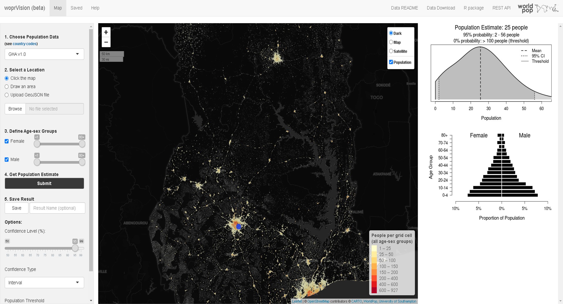
Figure 10.2: woprVision web application providing access to posterior predictions on an interactive web map (https://apps.worldpop.org/woprVision; select data ‘GHA v1.0’).
10.3.1 People per household
Analysis of residuals indicated that estimates of people per household were relatively unbiased (-6.4%) but predictions were very imprecise (76%) for individual households (r-squared = 0.05). This was expected due to the lack of location information from the household data. Despite imprecise household-specific predictions, the overall distributions of predicted household sizes were representative of household sizes within geographic units and settlement types (Fig. 10.3). The prediction intervals for people per household were robust with 96.8% of out-of-sample data falling within the 95% prediction interval and 69% falling within the 50% prediction interval.
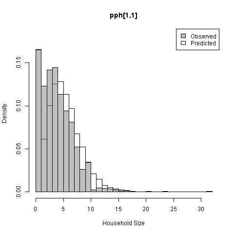
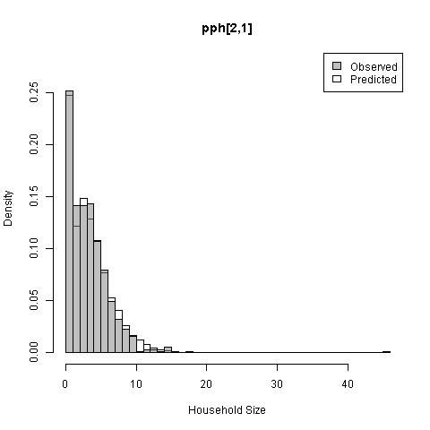
Figure 10.3: Distribution of people per household in geographic unit no. 1 for urban areas (left; t=1, g=1) and rural areas (right; t=2, g=1).
Estimates of \(\alpha_{t,g}\) (bias = 1.3%, imprecision = 19.2%) and \(\lambda_{t,g}\) (bias = -1.3%, imprecision = 8.3%) were much more accurate because they were estimated for larger spatial scales (geographic units \(g\)) with r-squared values of 0.88 and 0.93, respectively (Fig. 10.4). It is important to note that \(\alpha_{t,g}\) is the probability that a household contains only a single person and \(\lambda_{t,g}\) is the average number of people in a household other than the head of household. We did not assess the coverage of the prediction intervals for each of these parameters individually because they are component parts of a mixture distribution representing people per household, which was assessed above.
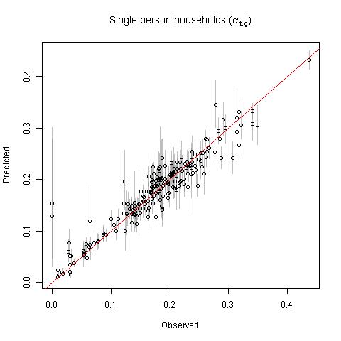
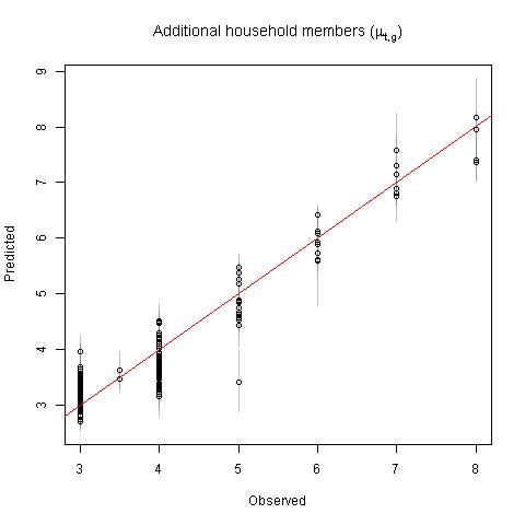
Figure 10.4: Observed versus predicted parameters for estimating people per household.
10.3.2 Age-sex structure
Estimates of \(\theta_{t,r,k}\) (i.e. proportion of population in each age-sex group) had an r-squared of 0.98 compared to out-of-sample data (Fig. 10.5; bias = -6.6%, imprecision = 18%). The slight negative bias was particularly apparent for estimates of adult males in some geographic units (see Appendix B). The 95% prediction intervals contained only 48% of out-of-sample data and the 50% prediction intervals contained only 21% of out-of-sample data. The underestimated prediction intervals may have resulted from the strong constraints of the Dirichlet distribution requiring the proportions to sum to one.
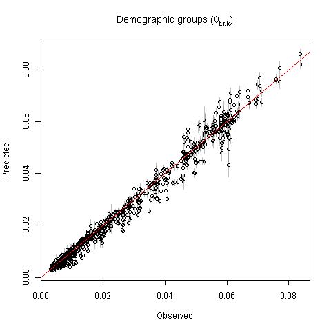
Figure 10.5: Observed versus predicted proportion of the population in each age-sex group. The plot shows all age-sex groups across all regions.
The population pyramids that resulted from the estimates of theta differed slightly between urban areas and rural areas (Fig. 10.6). Urban areas had a wider base indicating a higher proportion of children. Within settlement types, there were slight differences in population pyramids among geographic units (see Appendix B).
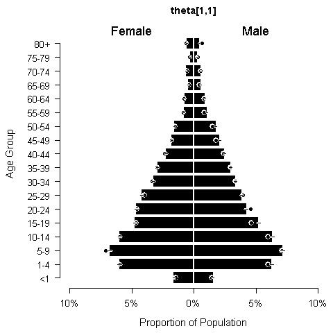
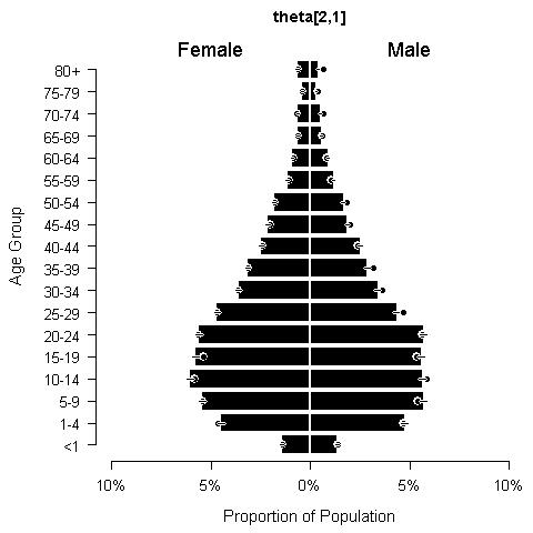
Figure 10.6: Population pyramid in region no. 1 for urban areas (left, t=1, r=1) and rural areas (right, t=2, r=1). Dots are observed out-of-sample data, while bars and their credible intervals are posterior predictions from the model.
Figures comparing model estimates of people per household and age-sex structure to out-of-sample observations (like Figs. 10.3 and 10.6) are provided in Appendix A for all geographic units.
10.3.3 Census projections
Model estimates of total population in each population unit \(u\) were comparable to the projected census totals used as input data for most areas (r-squared = 0.98), but there were significant divergences in two units (Fig. 10.7) where the census projections were likely significant underestimates that did not account for urban growth into these suburban/rural areas. One of the areas was on the north side of the city of Kumasi and the other was west of the city of Tamale (see results at https://apps.worldpop.org/woprVision; select data “GHA v2.0”).
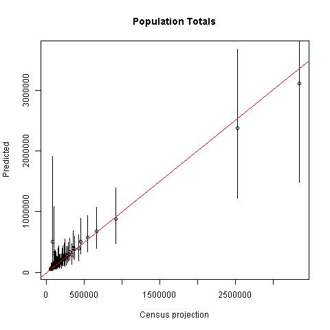
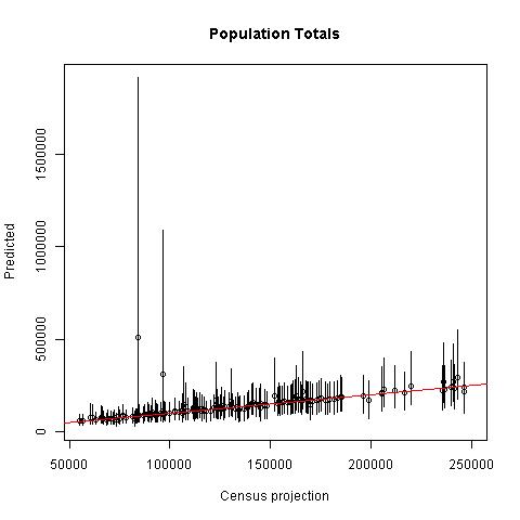
Figure 10.7: Census projections versus model predictions of total population sizes in 170 spatial units. The panel on the right is zoomed in to units with less than 250,000 people.
10.4 Discussion
The model is a hybrid between commonly used top-down and bottom-up approaches (Wardrop et al. 2018a) that are often used to map populations when complete census results are not available. It is similar to bottom-up approaches because it uses household-level survey data that do not have full coverage of the country and it is similar to top-down approaches because it uses projected census totals to constrain population estimates. Unlike other top-down approaches (Stevens et al. 2015a), this model enforces a “soft constraint” in which the population totals can deviate significantly from the census projections provided as input data if the weight of evidence from the rest of the model suggests the projections are inaccurate. This approach is unlike top-down or bottom-up approaches because it cannot use high-resolution geospatial covariates other than the count of buildings in each 100 m pixel.
This modelling approach produces high resolution gridded population estimates from publicly available census microdata that have been standardized across countries by IPUMS International (Minnesota Population Center 2019). The building footprints that are the other critical piece of data have been produced for 51 countries in sub-Saharan Africa (Ecopia.AI & Maxar Technologies, Inc. 2019-2021, Dooley et al. 2020a). This provides an opportunity to produce rapid population estimates for countries where both data sets are available. We achieved this by estimating the average number of households per building and the average number of people per household for urban and rural sub-national geographic units using a hierarchical Bayesian modelling approach. Importantly, the method accounts for uncertainty which can be significant for approaches like this that do not have detailed spatial information associated with the population data, which is the usual situation when using publicly available data.
This method cannot map variation in people per household or households per building with precision at the 100 m spatial scale because the specific locations of households are not available for the census microdata. The model estimates these parameters for urban and rural settlements in over 100 geographic units across the country, but it does not attempt to map variation within those units. It accounts for that variation as statistical uncertainty which results in the population estimates having fairly wide credible intervals. Because we used data from the 2010 Ghana census to estimate the number of people per household and the proportion of the population in each age-sex group for urban and rural settlements in various regions, we have assumed that the patterns of people per household and age-sex structure have not changed in these areas since 2010. This was a necessary assumption in the absence of more recent survey data, however the model can be updated when newer data become available.
We suggest labelling the population estimates as 2018 because this was the most common satellite image acquisition year (Fig. 10.8) for imagery used by Maxar Technologies and Ecopia.AI (Ecopia.AI & Maxar Technologies, Inc. 2019-2021) to derive the building footprints. The year of satellite images varied across the country from 2009 to 2019, depending on the exact location. Refer to the raster GHA_buildings_v1_1_imagery_year.tif (Dooley et al. 2020a) for a map of the imagery years of building footprints. We assumed that the building footprints represented all potentially residential buildings. We did not account for buildings that were missing from the building footprints or that have since been removed. We did not have quantitative measures of building footprint accuracy available to us.
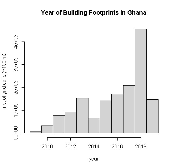
Figure 10.8: Distribution across Ghana of the year of building footprints (Ecopia.AI and Maxar Technologies 2020, Dooley et al. 2020).
We identified a few areas for improvement in this model. The credible intervals for the age-sex structure are not capturing the full range of variation. One potential solution may be to apply a hierarchical Dirichlet prior to constrain the population pyramids to share information among regions. The estimated distributions of people per household appeared not to fit the out-of-sample data for a few geographic units and this warrants further investigation, particularly to understand the effects of outliers on the one-inflated Hurdle model. It would also be helpful to conduct a formal sensitivity analysis to assess the influence of the informative prior that we used to quantify measurement error in the census projections.
In addition to these next steps to improve the method and better understand its nuances, it will be important to apply it across countries to understand how generalizable it is. Our intention for this approach is to apply it rapidly as a gap-filling measure while efforts are underway to acquire geolocated population data for population modelling to support development projects, planning for programs, and census preperations. The model’s estimates of people per household and households per building may also serve as a guide for setting these parameters in the peanutButter application (Leasure et al. 2020b) for countries where census microdata or other household surveys are not publicly available.
Note: The gridded population estimates for Ghana that were produced using the methods described in this chapter are available from the WorldPop Open Population Repository and they can be explored on a map using the woprVision web application (select “GHA v2.0”). Supplemental data for this chapter are available from http://doi.org/10.5258/SOTON/WP00686.
Contribution
This chapter was written by Douglas Leasure with oversight from Andy Tatem