7 Introduction to Small Area Population Estimation and Modelling (SAPEM)

This module focuses on small area population estimation, with information on both direct and indirect estimation methods, where the latter includes both top-down and bottom-up methodology. For this module, much of the relevant code is provided by the Book of Methods.

7.1 Small area population estimation

Small area estimates (SAE) of a population use statistical techniques and models to provide a reliable population number at smaller (granular) area units, where the areas or domains often correspond to geographic domains (e.g. school districts and health service areas) or to socio-demographic groups (e.g. age by gender groups and groups in poverty). This is often done using multiple data sources, for example, sample surveys, and auxiliary data which have wider coverage with geospatial covariates, administrative data and census data. Small area population estimation is both quick and cost effective.

SAE is needed, often as the focus of data collection systems is on the “big picture”, meaning that resulting estimates are reliable only to the highly aggregated levels such as national or regional levels, and not reliable for the smaller areas such as provinces or school districts. Additionally, granular or disaggregated data collection typically requires more resources, for example, more money, people and equipment, and often takes much longer. In many cases, limited resources are available, with time and financial constraints, so the granular data is not available, which is where SAE comes in useful. It should also be noted that there are challenges with traditional surveys, where census data is often very outdated (illustrated later in the module in Section 3. Indirect estimation).

There is a demand for SAE given the importance of granular data being used in policy-making and decision-making, such as economic policies, business planning and allocation of government funds.

There are two main methods to small area population estimation, direct estimation methods and indirect estimation methods, where the latter includes spatial statistical population models, for example, a bottom-up model.

For implementation of SAE in R, the following packages can be utilised.

• car: provides functions that are useful for assessing regression models, calculations around those models and graphics.
• sae: provides functions to obtain model-based estimates for small areas, for both (basic) direct and indirect estimation methods, among other useful functions.
• InformationValue: provides functions that assess the performance of classification models among other useful functions.
• rsq: provides functions that compute the generalised R-squared and partial R-squared statistics, and partial correlation coefficients for GLMs.

One of the problems with using satellite images for population size estimation is that satellite imagery does not always identify where there are buildings, for instance, when there is tree canopy covering a settlement. In this case, modelling is useful for better predicting the population size. A 2-step model solution is used as follows.

• Step 1: The relationships between the geospatial covariates and building intensity are exploited with a Bayesian hierarchical modelling framework. Estimates of building intensity across the entire area, including the areas under tree canopy cover, are obtained using the best fitting model.
• Step 2: The estimates of the building intensity obtained in Step 1 are then used to calculate population density. The relationship between population density and a set of geospatial covariates are explored within a Bayesian hierarchical modelling framework.

As discussed in previous modules, the form of linear and generalised linear models are as given below. The form of a generalised additive model (GAM) is also given for reference.

• Linear model (LM): \(Y_i = \beta_0 + \beta_1X_i + \epsilon_i\), where \(\beta_0\) is the intercept, \(\beta_1\) is the slope and \(\epsilon_i\) is the error term.
• Generalised linear model (GLM): \(g(\mu_i) = \beta_0 + \beta_1X_i\), where \(\beta_0\) is the intercept and \(\beta_1\) is the slope.
• Generalised additive model (GAM): \(g(\mu_i) = \alpha + \sum_{j=1}^K f_j(x_j)\) where \(g(\mu_i)\) is the mean function (for example, log, logit or identity), \(\alpha\) is the intercept and \(f_j(x_j)\) is the smooth function for continuous covariates.

Similarly, the following models are with a non-spatial random effect, \(v_i\), that does not describe any form of spatial dependence between the observations in the linear, generalised linear and generalised additive mixed models.

• Linear mixed model (LMM): \(Y_i = \beta_0 + \beta_1X_i + \epsilon_i + v_i\)
• Generalised linear model (GLMM): \(g(\mu_i) = \beta_0 + \beta_1X_i + v_i\)
• Generalised additive model (GAMM): \(g(\mu_i) = \alpha + \sum_{j=1}^K f_j(x_j) + v_i\)

However, these models are non-spatial, as they do not have a spatial random effect. The following models are spatial statistical models, given that they have a spatially varying random effect, \(v_i\), which varies in space as a result of spatial geography (where individuals live). This relationship is described using the statistical models that are usually distanced based or use neighbourhood matrices.

• Linear mixed model (LMM): \(Y_i = \beta_0 + \beta_1X_i + \epsilon_i + v_i\)
• Generalised linear model (GLMM): \(g(\mu_i) = \beta_0 + \beta_1X_i + v_i\)
• Generalised additive model (GAMM): \(g(\mu_i) = \alpha + \sum_{j=1}^K f_j(x_j) + v_i\)

It is important to check which geospatial covariates are significant, since as with non-spatial models and covariates discussed in Module 4, you only want to include significant geospatial covariates in the spatial statistical models. This can be done in R by following these steps:

1. Specify an appropriate GLM for the response with all the covariates included to obtain the model f1. In the example below, given that the data is count data, a Poisson distribution is used. For more information on why, see Module 4 Section 4: Generalised linear regression.

#specify appropriate GLM
f1 <- glm(pop ~., data = data_pop, family = poisson) #count data for Poisson 
#summary for the model
summary(f1)

2. Run a stepwise selection with the stepAIC() function with the MASS package. See Module 4 Section 7: Stepwise regression for more information on the stepAIC() function and stepwise regression.

#use stepAIC() for both ways stepwise regression
step_pop <- stepAIC(f1, scale = 0, direction = c("both"), trace = 1, 
                    keep = NULL, steps = 1000, use.start = FALSE, k = 2)
step_pop

3. Rerun the selected model and call it something else, for example, f2.
4. Check for multicollinearity through computing the Variance Inflation Factors (VIF) using the vif() function from the car package.

#use vif() to check for multicollinearity
vif_f2 <- vif(f2)

5. Retain only significant covariates with a VIF value of less than 5 (note: 5 is not always the chosen level of significance).

#select covariates with vif value of < 5
vif_f2[which(vif_f2 < 5)]

7.2 Direct estimation

Firstly, the domain of a survey specifies to which level precise and accurate estimates can be obtained. Then, suppose that the target population of the survey can be divided into \(M\) domains (\(D_1, \cdots, D_m, \cdots,D_M\)).

To estimate the population size of a small area (for example, the total number of people in poverty), direct (survey) estimation can be used. The characteristic of interest, \(y_j\) must be specified (for example, \(y_j=1\) if the sampled unit is classified as in poverty and \(y_j=0\) otherwise), with each sampling unit having an associated sampling weight, \(w_j\). The resulting direct survey estimate \(\hat{Y}\) can then be computed as the weighted sum of each characteristic of interest, \(y_j\), for each sampled unit \(j\) as follows.

\[ \hat{Y} = \sum_{j \in S} w_j y_j,\] where \(j\in S\) corresponds to each sampled unit in the survey.

If a domain is divided up into \(N\) sub-domains (\({SD}_1, \cdots, {SD}_n, \cdots, {SD}_N\)), the above formula can be adapted to compute the direct survey estimate for only the sampled units in sub-domain \(n\) by further restricting the summation to only include the sampled units within sub-domain \({SD}_n\) as follows.

\[ \hat{Y}_n = \sum_{j \in S, j \in {SD}_n} w_j y_j.\]

Whilst most direct survey estimators are unbiased, it is important to note that the sampling error of \(\hat{Y}_n\) can be high if there is not a suitable number of observations used in the calculation, i.e. if the sub-domain \({SD}_n\) is notably smaller than any of the survey domains \(D_m\).

A basic example of direct estimation can be found when trying to compute the average household size of a region. If you know the total population size and the number of households within a given region, then to estimate the average household size, you would divide the total population by the total number of households. This direct estimation is demonstrated in the code below.

#define total population
total_pop <- 149375
#define total household size
total_hh <- 29875
  
#compute average household size
ave_hh_size <- total_pop/total_hh
ave_hh_size

## [1] 5

For more information, see Asian Development Bank. For an example of implementation in R, see page 48. Alternatively, see the help files for the relevant packages. For example, the direct() function in the sae package can be used to compute the direct estimators of domain means, and the help file (?direct) provides the following example code to demonstrate the use of the function.

7.3 Indirect estimation

Maps are very important for population modelling. For example, if in a given country, the aim is to vaccinate as close to 100% of under 5s as possible against polio, maps can aid in the visualisation of how many under 5s there are and where they are in order to ensure the correct amount of vaccine is available for each area. Additionally, detailed maps of each region are required in order to plan vaccinator logistics and routes.

It is also important to consider the population at risk. To do this, supporting data on how many people there are and where they are, who they are and how do they move around is required.

In terms of population data, censuses are one of the best sources available for population levels and trends, for example, to visualise age pyramids. Census data also provides population demographic and socio-economic characteristics, in addition to information on housing characteristics and socio-economic inequalities, including poverty levels. Population data can be very valuable for many different uses. It can help with appropriate resource allocation and evidence-based policy making and planning, act as a support tool for public health planning and also aid in monitoring development goals. However, whilst valuable, there are many challenges faced with relying solely on census data for population data.

Whilst census data is very valuable, it is expensive and only collected once a decade, meaning that it can be very outdated with no way of monitoring the inter-censal years. This increases the need for more timely and detailed data. Registry and administration data can help fill these gaps, but they can be incomplete and unreliable in low-income settings, adding to the challenge of tracking progress towards development goals. Additionally, in some countries, even the most basic census, boundary and mapping data are lacking, where there have not been reliable censuses for many years, making it difficult to define a baseline and measure changes sub-nationally and regularly from this baseline. This means that additional resources are required, where new geospatial data sources can help compliment existing traditional sources to fill in the gaps and keep a sub-national focus.

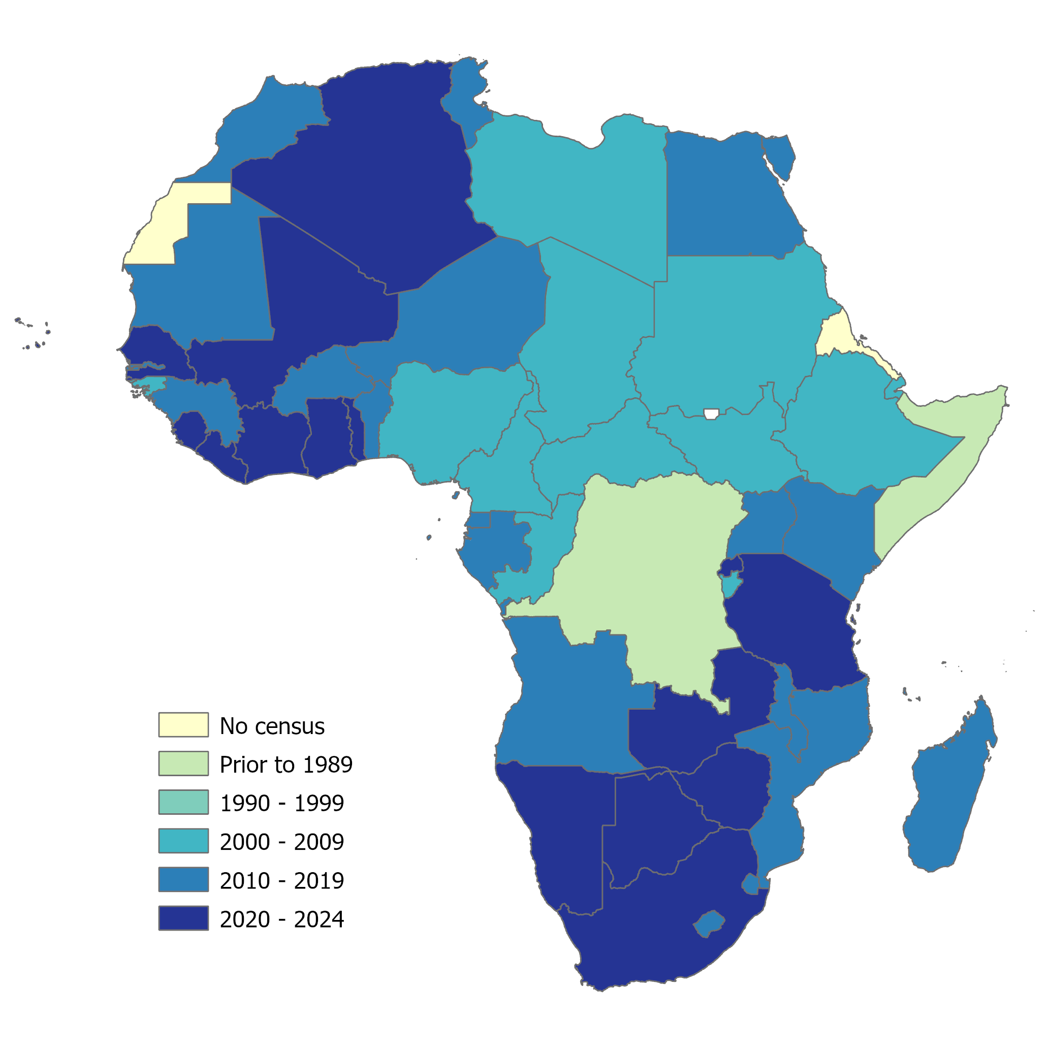
(#fig:africa census)Map of Africa illustrating scarcity of up-to-date census data (data correct as of December 2024)

These data sources can include geo-located household surveys, satellite, GIS and mobile phone data. All of these data sources are available more regularly than census data in inter-censal periods and are useful in low- and middle-income settings. However, whilst these sources are valuable in providing regular measurements and sub-national detail, they contain biases and gaps, therefore, it is important to integrate them with each other and more traditional data sources to draw on the strengths of each source and overcome some of the biases present.

In this context, population modelling is the process of combining aggregated/outdated census or survey data with a set of ancillary data to provide disaggregated population data. There are two main ways of doing this, top-down, where the admin-unit based census/official estimated counts are disaggregated, and bottom-up, where the census data is outdated/unreliable and so the satellite and mobile data is integrated with survey data. The bottom-up approach is independent of census data, and is more time-consuming and labour intensive, but can be the best approach when the census data is outdated and reliable. The top-down approach is the approach that forms most of WorldPop’s outputs at present.

7.3.1 Approaches for creating gridded population datasets

The data available changes at different stages of the census cycle, so the current stage of the cycle needs to be considered.

	Top-down	Bottom-up
Data sources	Census data. Administrative boundaries.	Survey data. Satellite imagery. Other ancillary data.
Directly following the census enumeration	Assumes complete spatial coverage. Assumes that the population totals for the administrative areas (e.g. EAs, wards, districts) can be spatially disaggregated.	If the spatial coverage is incomplete, the population enumeration areas can be used to predict the population in the incomplete areas.
During the inter-censal period	The projected population totals can be spatially disaggregated, however projections can become increasingly uncertain with the more time elapsed since the census was completed.	Activities such as listings from household surveys and census cartography that include complete (geolocated) listings of households or collect population count information can be used.
Advantages	It can be very straight-forward to implement. It can estimate the population distributions quickly.	Can capture the population distributions in more detail. When census data is unreliable, outdated or poor quality, can give more accurate estimates. Can estimate the population distributions in areas where there is no census data available.
Disadvantages	In areas where the population dynamics are complex or change rapidly, the accuracy can decrease. The accuracy depends on the quality of the census data - if the census data is outdated, unreliable or poor quality, the results can be inaccurate.	Takes more time, with more expertise needed, to produce the results. Requires more data than top-down for implementation.

7.3.1.1 Top-down

As mentioned above, this is the approach most commonly taken in WorldPop, focused on the disaggregation of admin-unit based census/official estimate counts. The approach combines the census population counts with the available geospatial covariates, disaggregating the population with a dasymetric approach, and producing gridded population estimates. The population data that is input for the top-down approach includes area-level population counts (e.g. wards and districts) with complete spatial coverage (generally from census/projections).

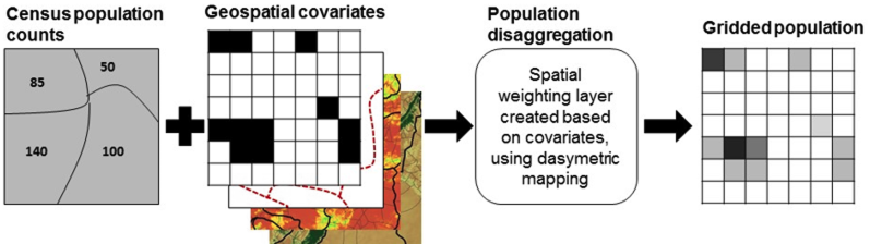
(#fig:top-down process)Illustration of the top-down approach process from Wardrop et al. (2018) PNAS

There are two main techniques for spatial disaggregation mapping, detailed as follows.

• Simple areal weighting: evenly redistributing aggregated population counts across all grid cells within each spatial unit.
  • Pycnophulactic redistribution: producing a smooth surface with disaggregated population values not changing abruptly across spatial unit boundaries.
  • Mask simple areal weighting: using a mask to define where, within each target unit, the input population counts must be evenly redistributed.
• Dasymetric disaggregation: redistributing input aggregated population counts across all grid cells within each spatial unit according to pre-defined weights (distributing population counts within selected boundaries through using covariate information such as land cover).
  • Mask dasymetric disaggregation: using a mask to define where, within each target unit, the input population counts must be daysmetrically distributed.

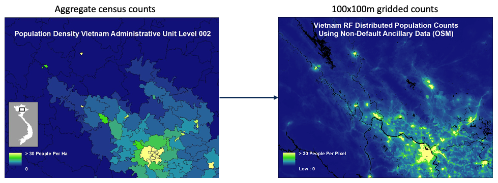
(#fig:disaggregation image)Visual example of top-down dasymetric approach

There are many benefits to producing gridded estimates, including aggregation flexibility and a fine-grained understanding of population variation. Also, a consistent grid enables easy comparison between areas and with other data themes/topics, for example, health data (location of health facilities, catchment areas, health zones, areas subject to floods).

There are many covariates available that depict contextual factors for top-down gridded population estimate. Some examples of these covariates are as follows.

Covariate type	Examples
Building patterns	Building counts Building density Building mean area Building total area
Residential patterns	Residential proportion Residential count Residential mean area Residential total area
Socio-economic patterns	Distance to marketplaces Distance to place of education Distance to local/main roads Distance to health providers
Environmental patterns	Slope Elevation Distance to bodies of water Distance to protected areas Distance to vegetation Distance to cultivated areas

The covariates used should relate to the spatial distribution of the population and available for the entire area. They should also include the geographical information on the location. Typically, covariates with continuous values are better than categorical values.

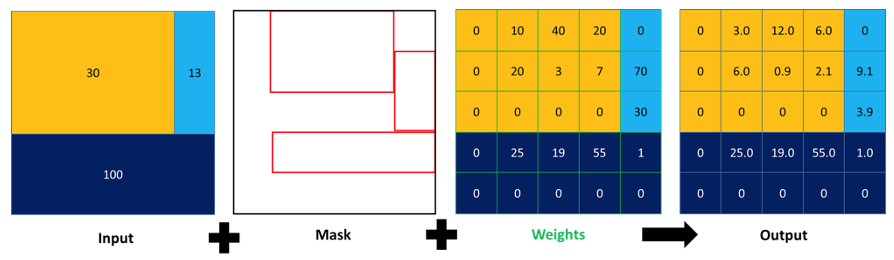
(#fig:mask dasymetric process)Illustration of the mask dasymetric disaggregation process

7.3.1.1.1 Random Forest model

The Random Forest algorithm is a commonly-used machine learning algorithm used construct individual regression trees in order to predict values of a response variable, for example, population density, for both categorical variables (classification) and continuous variables (regression). Prediction is done through using the relationship between the response and the geospatial covariates. It is important to note that Random Forest models are not good at extrapolating values.

Each of the trees constructed is trained using a random sub-sample of approximately 70% of the initial dataset. The final output is then the average prediction of all trees.

To use the Random Forest model in R, the package popRF developed for Random Forest-Informed Population Disaggregation can be used. It is published openly and descriptions available on the CRAN website. Previously, the dasymetric mapping method was very complex in terms of computation, with for example, different plug-ins or scripts from the weighting scheme to the disaggregation of the population counts. However, the popRF() function performs the entire modelling workflow automatically, making the process much simpler.

To use the popRF() function, the following arguments are required.

• pop: a tabular file containing the IDs of the sub-national areas and the corresponding total population.
  • The population counts file is a .csv file that contains two columns. One that contains the unique area IDs (the same as in the mastergrid) and another column that contains the corresponding population values.
• cov: at least one ancillary raster covariate dataset must be provided. If multiple covariates are used, then they need to be in a list format.
• mastergrid: the raster file representing the sub-national areas and corresponding tabular population count for those areas.
  • Mastergrid is also known as zonal data, and is the template gridded raster that contains the unique area IDs as their value.
  • Once the level of analysis is decided, it is recommended to create the mastergrid first.
• watermask: a binary raster file indicating the pixels with water (1) and no water (0).
  • Surface water does not need to be predicted and so a water mask raster is a required input.
  • If only building footprints are provided, the watermask can only contain 0s (i.e. non water) as the model will only predict to settled pixels.
• px_area: a raster file containing the area of each pixel in square meters.

To install the package directly from github, the function install_github() from the devtools package can be used as follows.

install.packages("devtools")
devtools::install_github("wpgp/popRF")

library("popRF")

Once the package is installed and loaded into R, the following are the main steps required to use the popRF() function.

1. Set the directory location of the inputs.
2. Create a list from the names and locations of the required covariates.
3. State the names and locations of the mandatory inputs.
4. Write the command line that executes the Random Forest application.

To assess the results from using the popRF() function, first it must be checked that the aggregated admin totals match the values in the population input file used. Also, it must be checked that the explained variance is sufficiently high (>80%), and remember that smaller-scale inputs improve the results a lot. Also, you should look over the results to see if there are any ‘weird’ shapes or patterns, and finally, check the results against a satellite image base layer.

For more information and implementation in R, see Chapters 17 and 18 of the Book of Methods.

7.3.1.1.2 Weighting layer

The weighting layer is used to divide up the population totals for each municipality into their enumeration areas (EA). This layer is created from predictive variables (geospatial covariates) related to population density, and associated with both the built and natural environment.

The weights represent the proportions of the population from each municipality (for \(j=1,...,J\)) that lives within EA \(i\) (for \(i=1,...,I_j\)), and can be calculated using the model predictions from the random forest model as follows.

\[ \text{weight}_i = \frac{\exp(\text{predicted}_i)}{\sum_{i=1}^{I_j}\exp(\text{predicted}_i)}\] where \(\text{predicted}_i\) is defined as the model prediction for EA \(i\) and \(I_j\) is defined as the total number of EAs in municipality \(j\).

Geospatial covariates are used as proxies of variation in population density and are spatially harmonised so that all variables have the same spatial resolution and grid cell alignment for the geospatial covariate stack. For the geospatial covariate stack, the subset of geospatial covariates that are most strongly correlated with population density should be selected. It is commonly found that the covariates derived from building footprints or residential information are strong predictors for population density. If there are any covariates which are unexpectedly high predictors for population density, those covariates can be removed to test whether they are influential/necessary.

7.3.1.2 Bottom-up

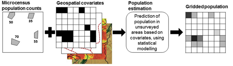
As mentioned earlier, the bottom-up methods are typically used when there is no recent (or appropriate) census data available in order to use the top-down approach. For the bottom-up methods, a sample of locations are chosen for which there is geolocated household survey data available. This data is then used in conjunction with geospatial covariates to fit a statistical model which estimates the population size in areas which were not sampled. In order to make the best use of the available data, for this approach, customised statistical models are applied, which also allow for probabilistic estimates of uncertainty.

The bottom-up modelling process is then as follows.

Step	Breakdown
Data collation, preparation and data analyses	Data cataloguing Data cleaning Variable description Variable preparation Shapefile cleaning Data visualisation Exploratory analyses Results presentation/discussion
Exploration of settlement data/ creation of geospatial covariates	Raster visualisation Raster cleaning Various raster analyses Covariate checks Correlation analysis Raster stacking Other activities
Development and exploration of various statistical model structures	Data integration Random intercept model development (STAN and INLA) Observation-level prediction Bayesian models with covariates (STAN and INLA) Observation-level prediction
Model selection, model validation, population prediction/ uncertainty quantification	Model checks and testing Model selection Cross-validation Population prediction Uncertainty quantification
Gridded population, estimates, model documentation, report and paper	Population gridding production Model outline documentation Report writing Manuscript preparation for scientific publication

(#fig:bottom-up process)Illustration of the bottom-up approach process from Wardrop et al. (2018) PNAS

For more in-depth explanations of the bottom-up methods and implementation in R, see Chapters 5, 6 and 7 of the Book of Methods. A summary of the key types of input data required as explained in the Book of Methods is given below.

There are a few key types of input data for bottom-up methods, these are as follows.

• Population data
  • Should include enumerated population counts for enumerated areas only (at cluster or geolocated household level).
  • Ideally includes a polygon shapefile with the boundary of each enumeration area and the total population within each area.
  • Additional (optional) information collected during census and surveys such as point locations of buildings and/or households within enumeration areas can be useful for providing higher resolution information.
  • Obtained from partial census results, microcensus surveys designed for population modelling and pre-survey listing data from routine household surveys
• Settlement map
  • Used for identifying where residential structures are located/exist via building locations (points), building footprints (polygons) and/or gridded maps identifying pixels that contain buildings (raster).
  • May classify areas into different settlement types.
  • Additional (optional) information for each building such as building area, height and use can be beneficial for population modelling.
  • Obtained from satellite imagery, pre-census cartography, building points and footprints and gridded derivatives of building footprints.
• Geospatial covariates
  • Spatial datasets with national coverage focused on variables which are likely to have some correlation to the population density.
  • Common geospatial covariates include road networks, night-time lights, locations of public facilities (e.g. hospitals or schools).
  • To ensure that the accuracy of the population estimates is as high as possible, the covariates used in the estimation should be highly correlated to the population density (good quality covariates) and has comprehensive national coverage.
• Administrative boundaries
  • May include regions, states (provinces), divisions and sub-divisions.
  • Administrative units are often nested within each other.
  • If there are population totals for each administrative unit, they can be used to summarise model results.

7.4 Useful resources

• Small area estimation: Introduction to Small Area Estimation Techniques
• popRF: WorldPop tutorial
• Top-down: Book of Methods
• Top-down: WorldPop tutorial
• Bottom-up: Book of Methods