11 Age-Sex Disaggregation
This is the final module and covers disaggregation of population totals by age-sex proportions for instances where there is age-sex data available as well as instances where there isn’t.
11.1 Disaggregation of population totals by age-sex proportions
Data disaggregation can be defined as the process of breaking data down into some predefined sub-categories and is helpful in the understanding of disparities and targeting interventions.
Two common sub-categories are age and sex. Age-sex disaggregation is of importance for several reasons. Firstly, it aids in the ability to make informed decisions for specific age and sex groups for policy making. Secondly, it can help with the effective allocation of resources, by allocating resources based on the specific needs of different groups of individuals. Finally, it is beneficial for monitoring and evaluation of different programmes through assessing the impact and progress of each programme.
There are three main methods for age-sex disaggregation, given as follows.
- Surveys and censuses: data is collected from questionnaires such as the Demographic and Health Surveys (DHS) and censuses.
- Administrative records: Data is collected from different institutions such as enrolment records from schools or patient data from hospitals.
- Sample surveys: data is collected from a representative sample such as the labour force surveys or health surveys.
Several challenges are faced when conducting age-sex disaggregation. Issues can arise if the data is of poor quality, for example, if the data available is incomplete or inaccurate. Additionally, there can be privacy concerns regarding how to ensure the confidentiality and security of the data. The last main concern is that of constraints on the resources, as often funding is limited as well as a constrained technical capacity.
Data availability is another thing that needs to be considered as there are two cases of data availability, either there is age-sex data available, or there isn’t.
11.1.2 Available age-sex data
If the age-sex data is available, there are statistical methods and techniques available to refine the age distributions, which are particularly useful when dealing with incomplete or grouped data. For this, the DemoTools package in R is of use, along with the following methods.
- Penalised Composite Link Model (PCLM): uses a penalised likelihood approach to distribute aggregated age data into narrower age intervals. This is particularly useful to refine the age distributions from census or survey data when the intervals of age are wide.
- Sprague Multipliers: often used in demographic studies when the population data needs smoothing by interpolating the age distributions from broad age intervals into single-year intervals.
- Beers’ Ordinary and Modified Methods: creates detailed age distributions with single-year intervals from grouped data by fitting a polynomial curve to the existing age distribution.
- Karup-King Method: fits a polynomial curve to the age distribution to distribute the population counts into narrower age categories.
- Zigzag Method: often improves the accuracy when used alongside other methods as it is a smoothing technique that adjusts the age data to reduce the number of irregularities.
11.1.2.1 Age-sex disaggregation
When there is age-sex data available, the data can be disaggregated with the function given later in this section. However, first, the required functions of raster and peanutButter need to be loaded. An optional package is the tictoc package which can be used to time how long the end function takes to run.
#load packages
library(tictoc)
library(raster)

#devtools::install_github('wpgp/peanutButter')
library(peanutButter)
Then, the data needs to be input into the R environment and settings specified.
#input data
population <- raster(paste0(data_path, "pop_hat_total.tif"))
dept <- raster(paste0(data_path, "CMR_Department.tif"))
proportions <- read.csv(paste0(data_path, "CMR_2020_agesex.csv"),
stringsAsFactors = FALSE)
#settings
country <- 'CMR' #country code
version <- 'v1_0'
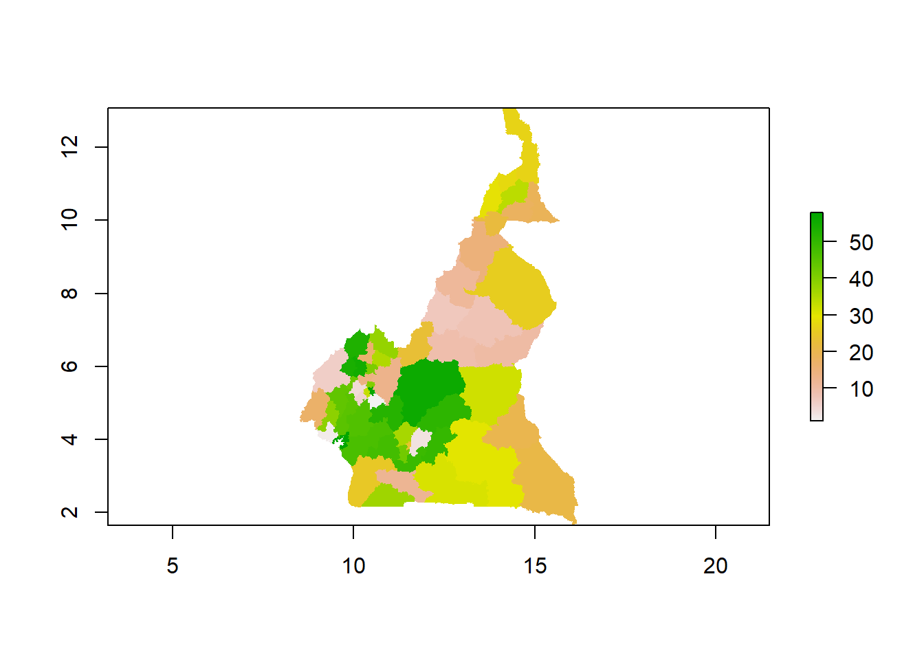
woprname <- paste0(country, '_population_', version,'_')Once the data has been input, the department raster can be plotted to aid in visualising the dataset.
Before creating the function which performs the age-sex disaggregation itself, a function that creates a population grid for each of the age-sex groups, returning the corresponding group population can be created, as seen below.
Within the age-sex disaggregation function, the demographic() function from WorldPop’s peanutButter package is required. Whilst the function can be called with peanutButter::demographic(), for understanding how age-sex disaggregation works, it is important to understand the key functions. Therefore, the required arguments, key steps and a breakdown of the function itself are given below.
The arguments that need to be included in the function are as follows.
population: the raster file for the population (populationin the Cameroon example).group_select: the group which you wish to create the population grid for (groupin the Cameroon example).regions: the raster file for the regions (deptin the Cameroon example).proportions: the.csvfile for the proportions of each age-sex category (`proportions in the Cameroon example).
Within the function itself, there are 6 key steps.
- Format the proportions data by appropriately naming the first column
idand renaming each of the rows to be the correct ID number. - Sum the proportions for the selected group. If the ‘group’ is one age-sex combination, then there will be only one proportion available. If multiple age-sex combinations are selected, sum the individual corresponding proportions for an overall proportion of that group.
- Reduce the columns to contain only the ID numbers and the relevant proportions.
- Save the raster coordinate system with the
crs()function and extract the minimum and maximum x and y coordinates of the selected region to save the extent of the boundary. - Convert the
regionsraster and proportions to a matrix, then rasterise the group proportions. - Compute the age-sex population through multiplying the population by the group proportion.
#function to create population grid for each age-sex group
demographic <- function(population, group_select, regions, proportions){

  #format proportions
  names(proportions)[1] <- 'id'
  row.names(proportions) <- proportions$id

  #sum the proportions for the selected group
  if(length(group_select)==1){
    proportions$prop <- proportions[, group_select]
  } else {
    proportions$prop <- apply(proportions[,group_select], 1, sum, na.rm=TRUE)
  }

  #reduce cols
  proportions <- proportions[, c(1, ncol(proportions))]

  #save the raster coordinate system
  crs1 <- raster::crs(regions)
  #save the extent of the boundary (minimum and maximum x and y coordinates)
  ex1 <- raster::xmin(regions)
  ex2 <- raster::xmax(regions)
  ex3 <- raster::ymin(regions)
  ex4 <- raster::ymax(regions)

  #convert the regions raster to matrix
  regions <- raster::as.matrix(regions)

  #proportions to matrix
  group_proportion <- regions
  group_proportion[] <- NA
  for(id in proportions$id){
    group_proportion[which(regions == id)] <- proportions[as.character(id),
                                                        'prop']
  }

  #rasterise the group proportions
  group_proportion <- raster::raster(group_proportion, crs = crs1, xmn = ex1,
                                     xmx = ex2, ymn = ex3, ymx = ex4)
  #calculate age-sex population
  group_population <- population * group_proportion
  return(group_population)
}
The next step is to create the age-sex disaggregation function itself. For ease of understanding, the required arguments and the key steps of the function are given below, before the details of the function itself. It is important to note that the population information for each age-sex category is of interest, so a full breakdown of the population is needed. However, it is also of interest in many instances to have information on children (both sexes) under the age of 1, under the age of 5 and under the age of 15 in addition to females of reproductive age between 15 and 49, so the population information for these specific groups is also computed within the function.
The required arguments for the age-sex disaggregation function (woprAgeSexRasters()) are as follows.
country: the country code for the country that the dataset is for.version: the current version/copy of the disaggregation being carried out.outdir: the out directory where the results will be saved.population: the raster dataset for the population.regions: the raster dataset for the regions.proportions: the.csvfile for the proportions of each age-sex category.
The key steps within the age-sex disaggregation function are.
- Create the out directory with the
dir.create()function. - Create a variable that contains the names of each age-sex category (group).
- Iterate between each of the groups, performing the
demographic()function for each group, saving the results as a raster with thewriteRaster()function from therasterpackage. - Compute the population information through stacking the age-sex for each of the other groups of interest (all children under 1, under 5 and under 15 as well as females from age 15 to 49).
#age-sex disaggregation function
woprAgeSexRasters <- function(country, version, outdir, population,
                              regions, proportions){
  #create out directory
  dir.create(outdir, recursive = TRUE, showWarnings = FALSE)
  woprname <- paste0(country, '_population_', version, '_agesex_')

  #create the groups for the age-sex combinations
  groups <- c(paste0('f', c(0, 1, seq(5, 80, 5))), #female + age combinations
              paste0('m', c(0, 1, seq(5, 80, 5)))) #male + age combinations

  #iterate between each of the groups
  for(group in groups){
    #create the out file path
    cat(paste0(group, '\n'))
    outfile <- file.path(outdir, paste0(woprname,group, '.tif'))
    if(!file.exists(outfile)){
      #create and save a raster that contains the demographic information
      #for each group
      raster::writeRaster(x = demographic(population = population,
                                          group_select = group,
                                          regions = regions,
                                          proportions = proportions),
                          filename = outfile,
                          overwrite = TRUE)
      }
  }

  #create the raster files for all children (both sexes) under age 1
  cat('U1 \n')
  agesex_stack <- raster::stack(file.path(outdir, paste0(woprname,c('m0', 'f0'),
                                                         '.tif')))
  result <- raster::stackApply(agesex_stack, raster::nlayers(agesex_stack),
                               fun = sum)
  result[is.na(population)] <- NA
  raster::writeRaster(result, file.path(outdir, paste0(woprname, 'under1.tif')),
                      overwrite = TRUE)
  rm(agesex_stack, result); gc()

  #create the raster files for all children (both sexes) under age 5
  cat('U5 \n')
  agesex_stack <- raster::stack(file.path(outdir,
                                          paste0(woprname,c('m0', 'f0', 'm1',
                                                            'f1'), '.tif')))
  result <- raster::stackApply(agesex_stack, raster::nlayers(agesex_stack),
                               fun = sum)
  result[is.na(population)] <- NA
  raster::writeRaster(result, file.path(outdir, paste0(woprname, 'under5.tif')),
                      overwrite = TRUE)
  rm(agesex_stack, result); gc()

  #create the raster files for all children (both sexes) under age 15
  cat('U15 \n')
  agesex_stack <- raster::stack(file.path(outdir,
                                          paste0(woprname,c('m0','f0','m1','f1',
                                                            'm5','f5','m10',
                                                            'f10'), '.tif')))
  result <- raster::stackApply(agesex_stack, raster::nlayers(agesex_stack),
                               fun = sum)
  result[is.na(population)] <- NA
  raster::writeRaster(result, file.path(outdir, paste0(woprname,
                                                       'under15.tif')),
                      overwrite = TRUE)
  rm(agesex_stack, result); gc()


 #create the raster files for females aged 15 - 49
  cat('F15-49 \n')
  agesex_stack <- raster::stack(file.path(outdir, paste0(woprname,
                                                         paste0('f',
                                                                seq(15,45,5)),
                                                         '.tif')))
  result <- raster::stackApply(agesex_stack, raster::nlayers(agesex_stack),
                               fun = sum)
  result[is.na(population)] <- NA
  raster::writeRaster(result, file.path(outdir, paste0(woprname, 'f15_49.tif')),
                      overwrite = TRUE)
  rm(agesex_stack, result); gc()
}
Finally, with the necessary packages installed, data set-up and functions defined, the age-sex disaggregation function can be applied to the chosen dataset, in this case the Cameroon data. Whilst it is not necessary to time how long the function takes to complete, since it does take a long time to finish running due to the large size of population datasets and rasters, it can be of interest to use the tic() and toc() functions to see how long it takes for the function to finish running.
11.2 Useful resources
- Aggregate demographic analysis: DemoTools
- Penalised Composite Link Model: Efficient Estiamtion of Smooth Distributions From Coarsely Grouped Data
- Sprague Multipliers: Estimating school-age populations by applying Sprague multipliers to raster data
- Beers’ Ordinary and Modified Methods: Create the Beers ordinary or modified coefficient matrix
- Karup-King Method: Karup-King-Newton method of population count smoothing
- Zigzag Method: Smoothing with DemoTools
- peanutButter package: WorldPop GitHub
- peanutButter package: peanutButter: An R package to produce rapid-response gridded population estimates from building footprints, version 0.1.0