1 Basics of R Programming

This module is ideal for individuals who have little to no experience with R, and those who would like a reminder. It contains the basics for getting started with R, beginning with how to install R on your computer, and understanding the key aspects of the software. Lastly, Module 1 gives an introduction to using R, including information on the basic operations, functions, and data structures.

1.1 Overview of R

R is a free, open source statistical programming language and environment used for statistical computing and has a wide range of graphical facilities for data analysis. Its uses also include (but not limited to) the following:

Data manipulation - e.g. extract, clean, store, process, …
Calculations (simple and complex) - e.g. addition, subtraction, …
Data visualisation - e.g. charts, line graphs, maps, exploratory analysis, …
Statistical and data analysis - e.g. regression, t-tests, correlation, …
Machine and deep learning - e.g. modelling, cross-validation, descriptive statistics, …
Reporting and creating documents (using Markdown and LaTeX) - e.g. reports, presentations, reproducible research, …
Mapping (Geographic Information System, GIS) - e.g. interactive visualisation, population size estimation,…

Getting started with R

Downloading R and RStudio

R can be downloaded on Windows, Mac and Linux from R-Project.org. Select the link to download for the correct operating system for your computer.

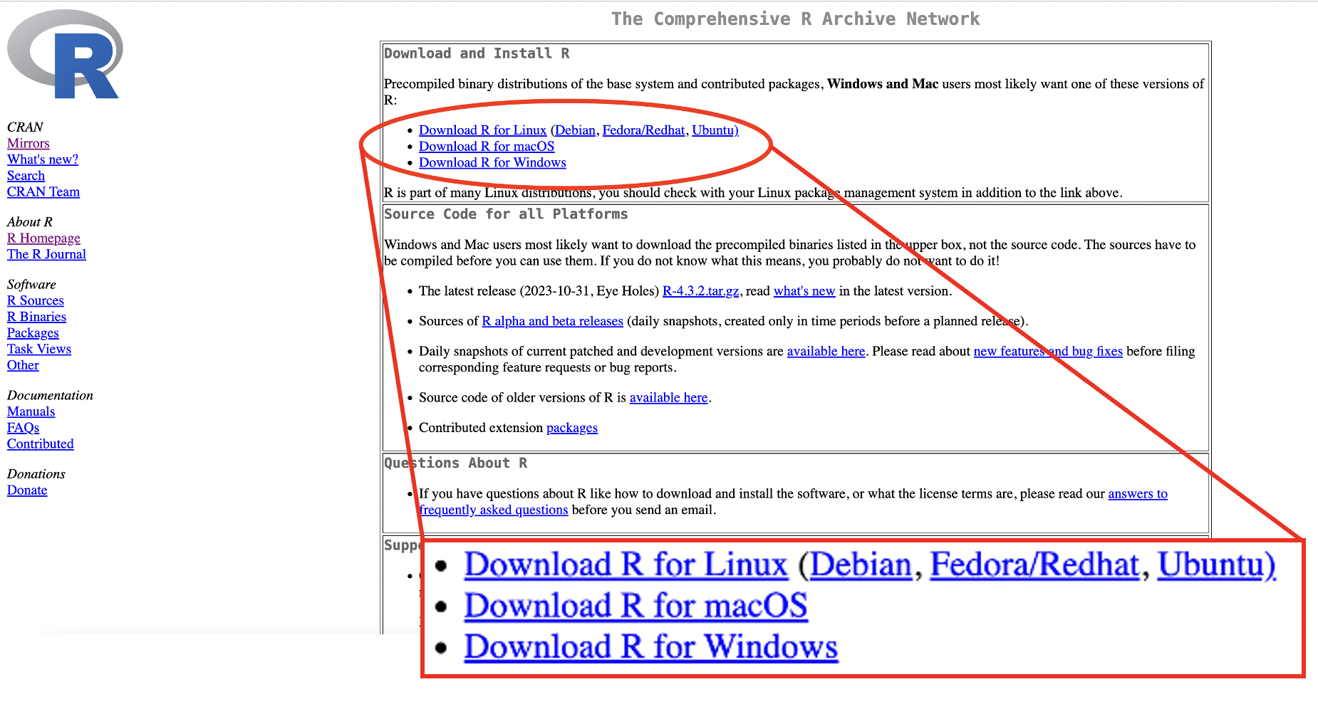
Figure 1.1: R download webpage

For Windows, click “install R for the first time”.

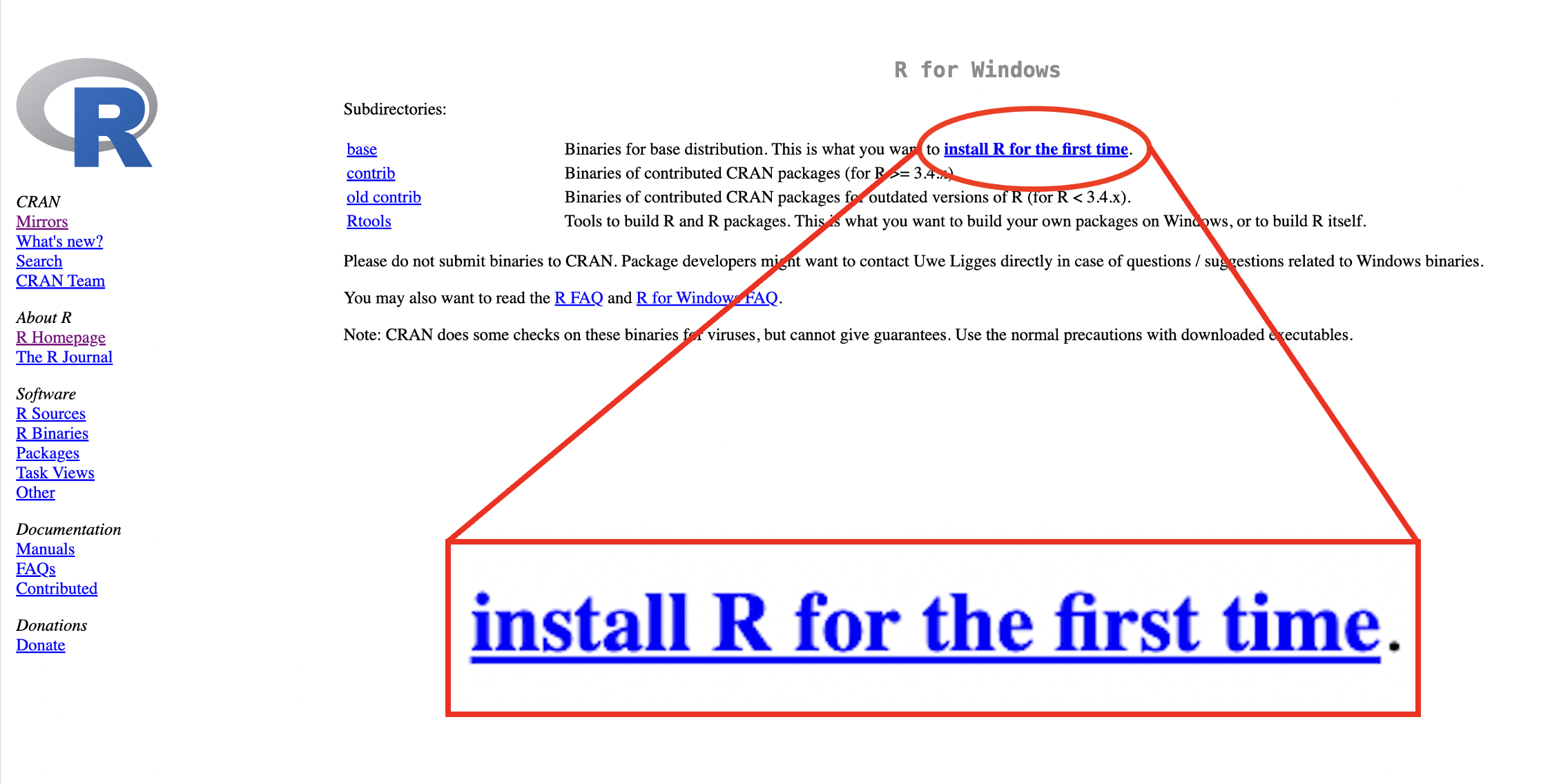
Figure 1.2: R download webpage: Windows

For macOS, click the correct download package for your Mac’s software version.

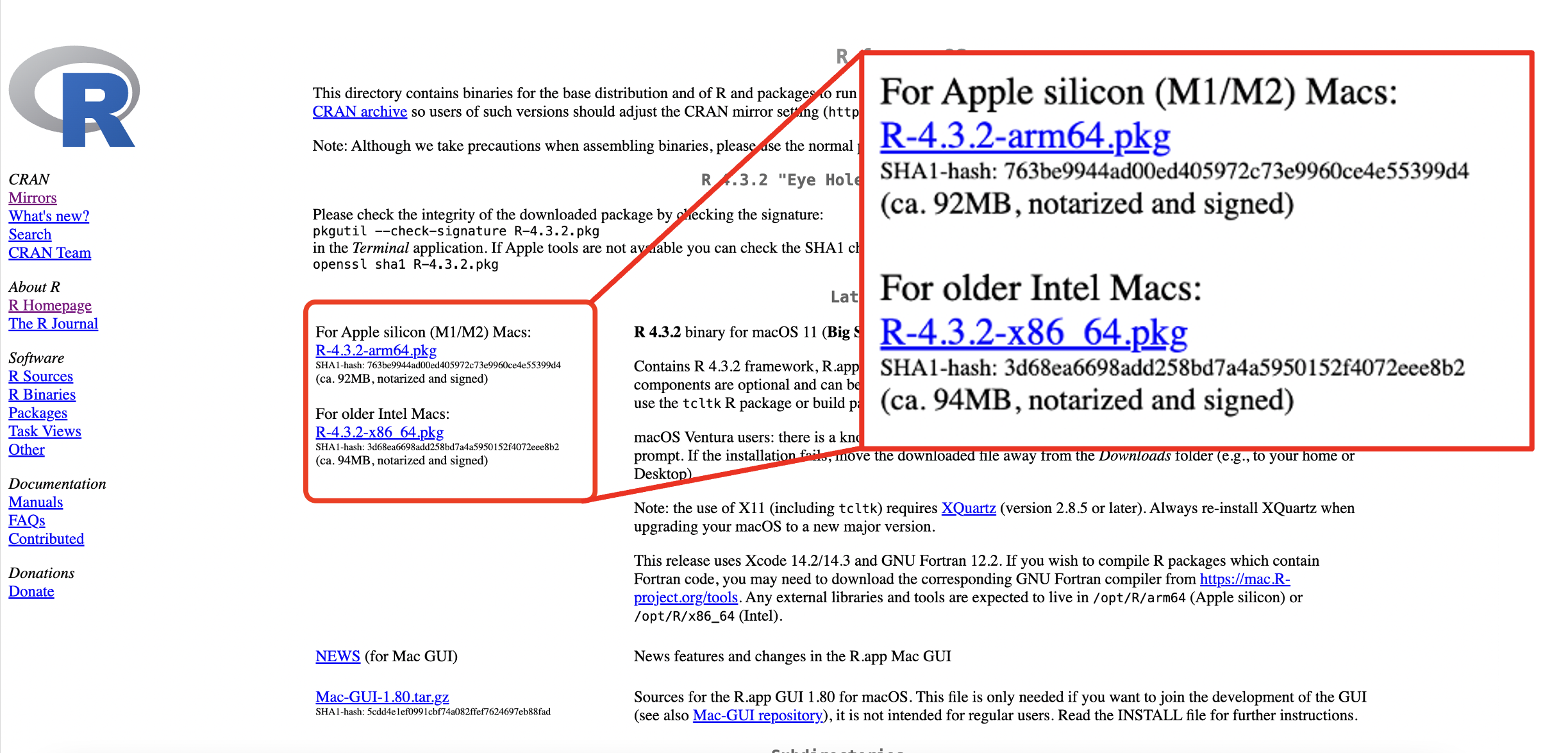
Figure 1.3: R download webpage: macOS

R does not have a particularly user-friendly graphical user interface (GUI). RStudio is a capable and free GUI add-on for R with improved functionality and usability. It can be downloaded from Postit.co. The webpage for downloading RStudio detects whether the operating system is Windows or macOS (or Linux), so the correct operating system does not need to be selected.

For Windows users, the webpage will look like the image below.

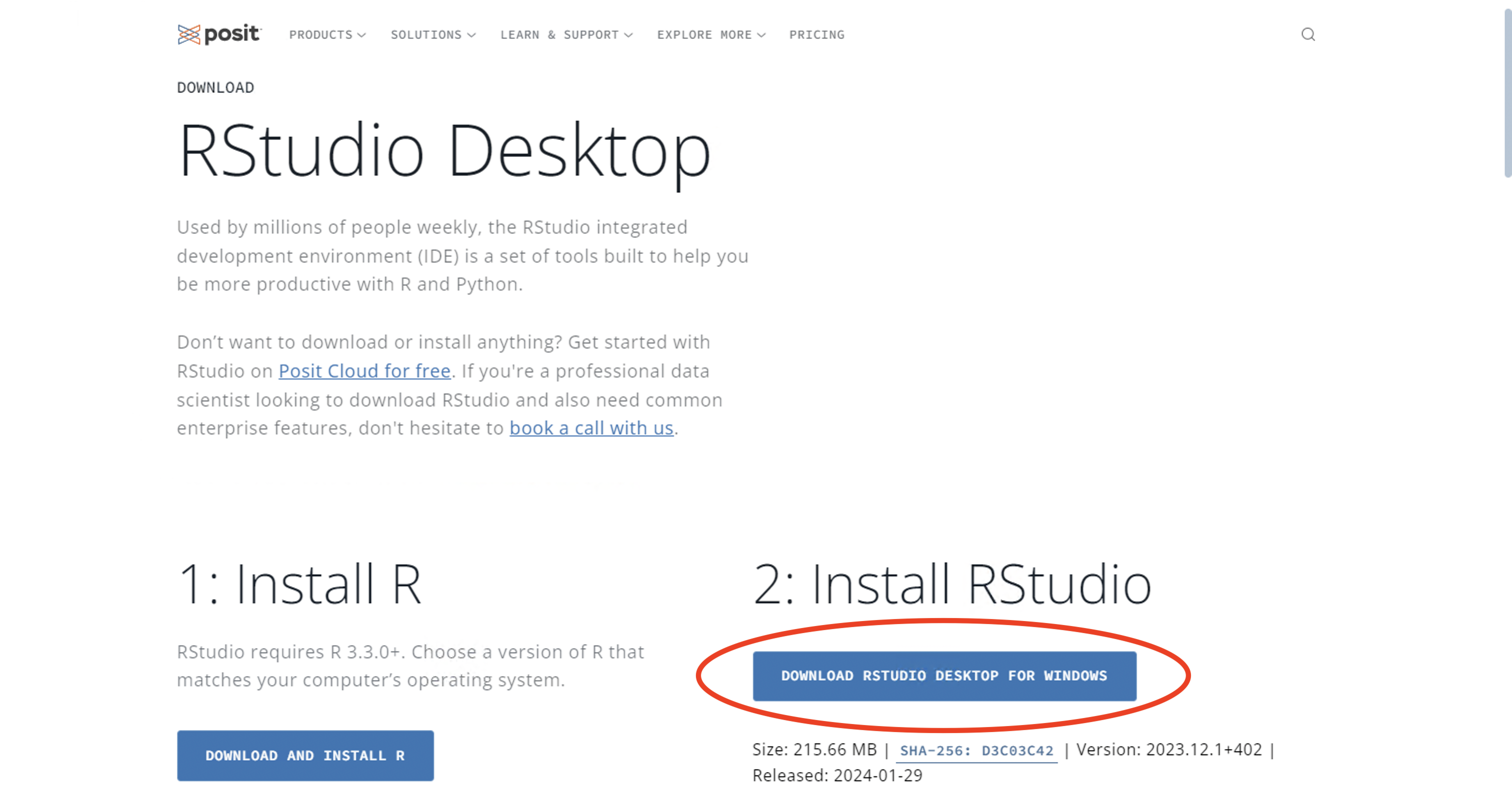
Figure 1.4: RStudio download webpage: Windows

For macOS users, the webpage will look like the image below.

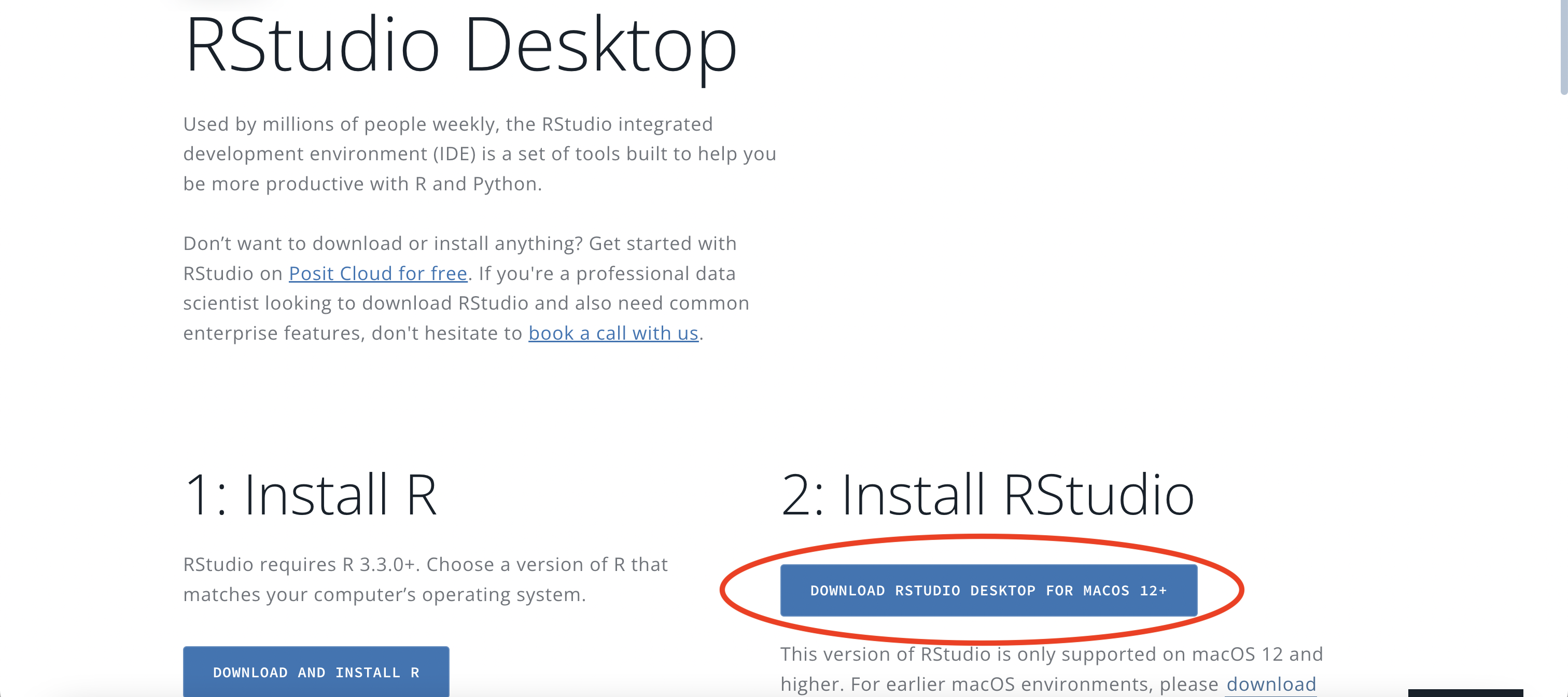
Figure 1.5: RStudio download webpage: macOS

Once “Download RStudio desktop” has been selected, the preferred version of RStudio can be selected, e.g. 2023.03.1+446, and the installation process can be followed once the download is complete.

To check both R and RStudio are installed on the computer, search for “R” and “RStudio” in the search bar of the computer. Once both are installed, the process is complete and they can be used.

Note: RStudio is just one example of R GUI, others are available such as Positron.

Features of the R GUI environment

When opening R, the user interface should have a window open for the console, where calculations can be made and results will be printed. It should look something like the image below.

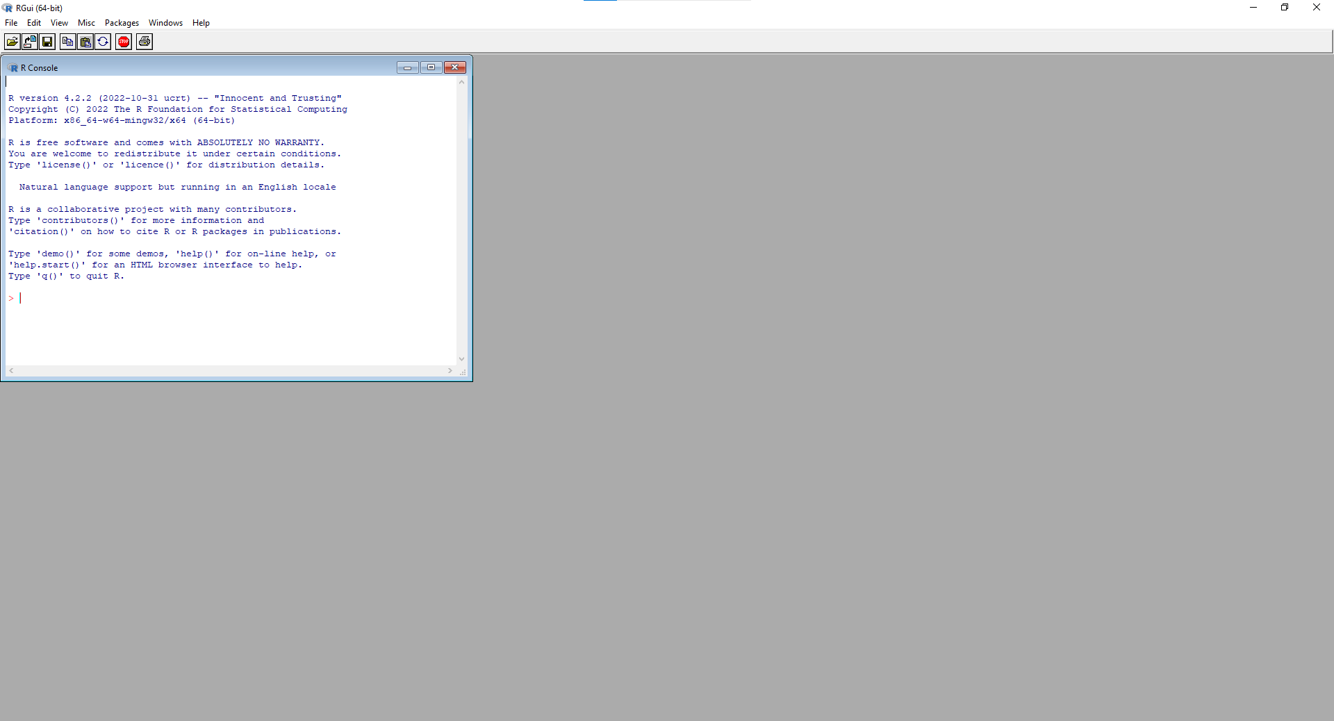
Figure 1.6: R GUI upon opening

Additional windows can be opened, such as windows for scripts to code in and windows to display plots, seen in the image below.

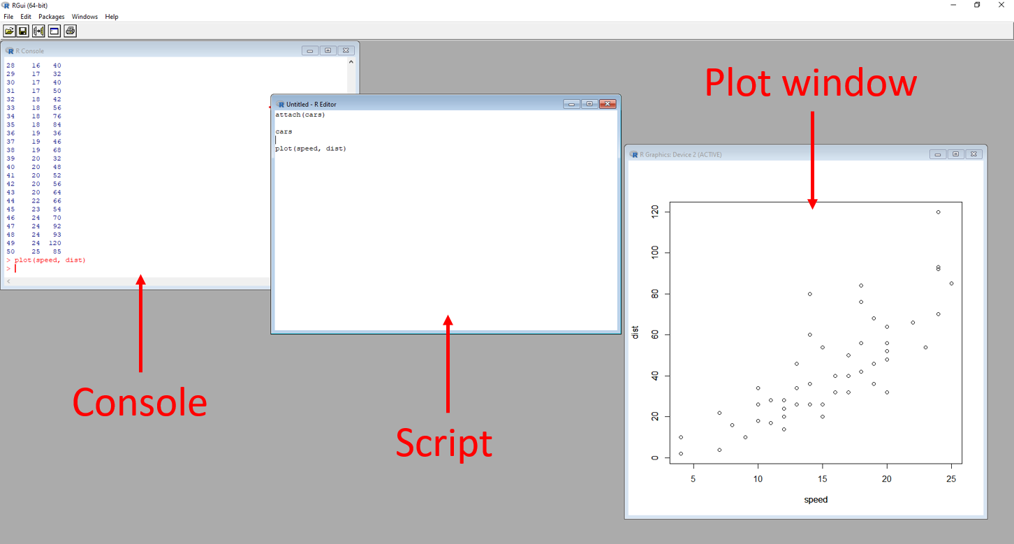
Figure 1.7: Annotated R GUI

Features of the RStudio environment

The user interface for RStudio is more efficient, with designated panes for displaying different information all at once in a much more convenient way.

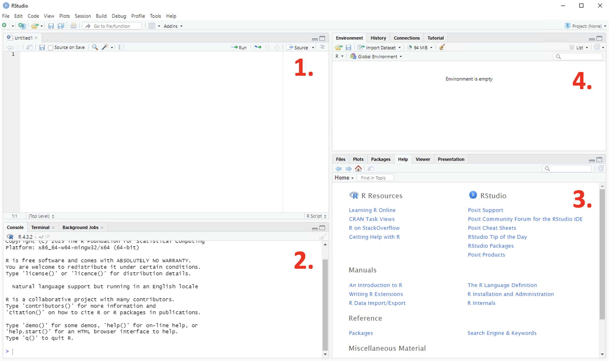
Figure 1.8: Annotated RStudio GUI

There are four panes as seen in the figure below:

Script - this pane is only present once a script has been created
Console - where numerical output will be returned
Viewer - computer files, plots, packages, help files, reports and presentations can be viewed here
Environment - any objects that have been created are present in the environment and can be cleared by clicking on the ‘broom’ icon toward the centre of the toolbar

See the image below for assistance in navigating the key aspects of the RStudio GUI.

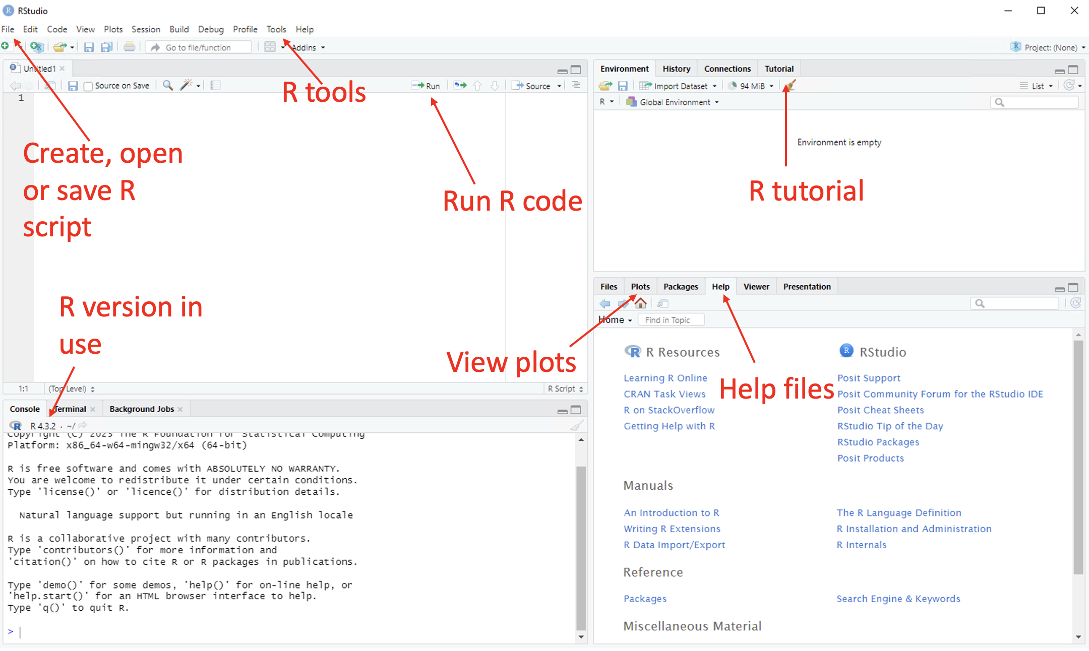
Figure 1.9: Annotated RStudio GUI

Creating, opening and saving R scripts

Whilst commands can be typed directly into the console, it is difficult to keep record of what has been run to ensure the code is reproducible and inconvenient when typographical mistakes are made. Utilising a script solves these issues, with the ability to make changes to and save the code written.

In RStudio, to open a new script, use the main toolbar and follow File > New File > R Script and pane 1 will appear. If a script is already present, it will open the new script in a new tab in the pane.

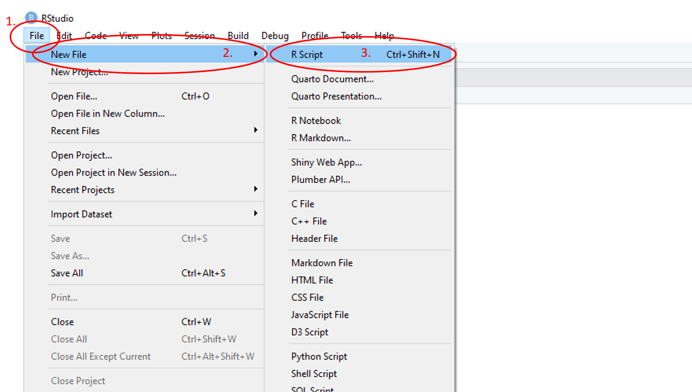
Figure 1.10: Annotated RStudio GUI: New script

To run the code from a script, highlight the desired line(s) to run and click Run on the script pane at the top right. Alternatively, keyboard short cuts can be used to run the code, press Control + Enter on Windows or Command + Enter on Mac. If code is run without highlighting any lines, only the current line (where the cursor is) will be run.

To open an existing R script, use the main toolbar and follow File > Open File then navigate to the desired R script in the files pop-up window.

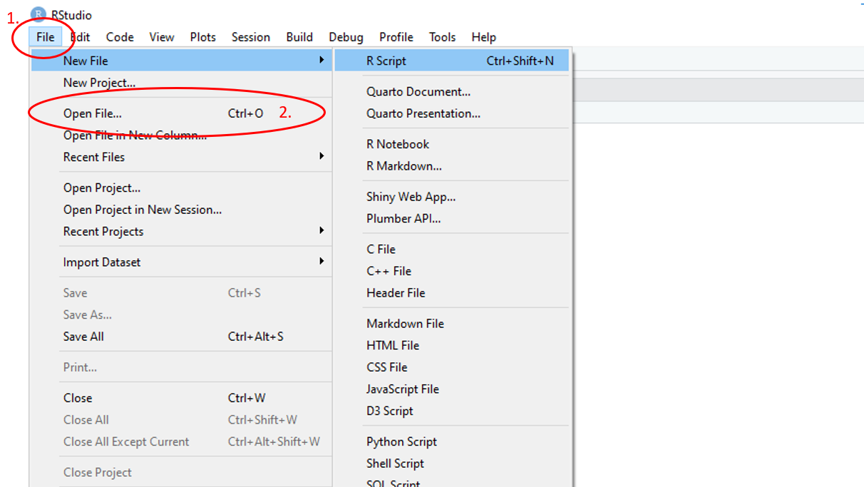
Figure 1.11: Annotated RStudio GUI: Open script

To save an R script, use the main toolbar and follow File > Save As and navigate to the desired location in the pop-up file directory window and name the script. To save updated versions of the script, use the main toolbar and follow File > Save

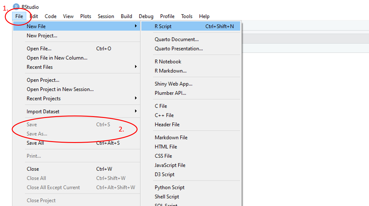
Figure 1.12: Annotated RStudio GUI: Save script

1.1.1 Getting and setting the working directory

The working directory is the folder on the computer where RStudio will access data and files from and/or save data to without any extra commands or steps. To avoid data and files being saved in an unknown location as well as to allow RStudio to access the data, it is important to know the working directory of your R session.

To check the location of the working directory, use the function getwd(). In the console, the working directory file path name will be printed.

To set the working directory, you use the function setwd(“location of your data folder”) and include the file path name in the parentheses.

Alternatively, the main toolbar menus can be used to set the working directory following the steps below, also demonstrated in the figure below:

Click on “Session”
Navigate to “Set Working Directory”
Navigate to “Choose Working Directory”
Select in your computer where you would like your R session files saved

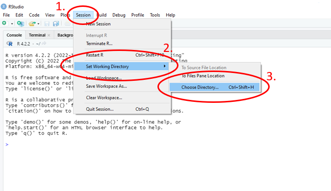
Figure 1.13: Annotated RStudio GUI: Set working directory

1.1.2 Creating, opening and saving R projects

When working with files in R, it is imperative that the working directory is set at the start of each script in order for R to be able to access the files. However, when working on different computers or working collaboratively with others, the file path will change leading to reproducibility issues.

An R Project is essentially a reproducible working directory, preventing the need to use the function setwd() in each script through having all of your work in a self-contained folder with a designated .Rproj file which can be opened and run seamlessly by anybody who has access.

To create an R project, use the main toolbar and follow the path File > New Project… > New Directory > New Project, give your directory a name and then click on Create Project.

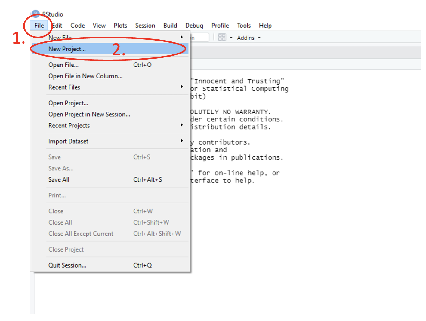
Figure 1.14: Annotated RStudio GUI: Create project

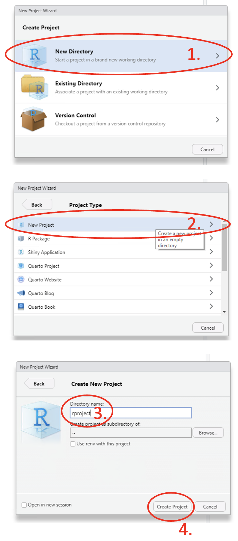
Figure 1.15: Annotated RStudio GUI: Create project

To open an existing R project, use the main toolbar and follow the path File > Open Project… > and select the desired project from the pop-up file directory window.

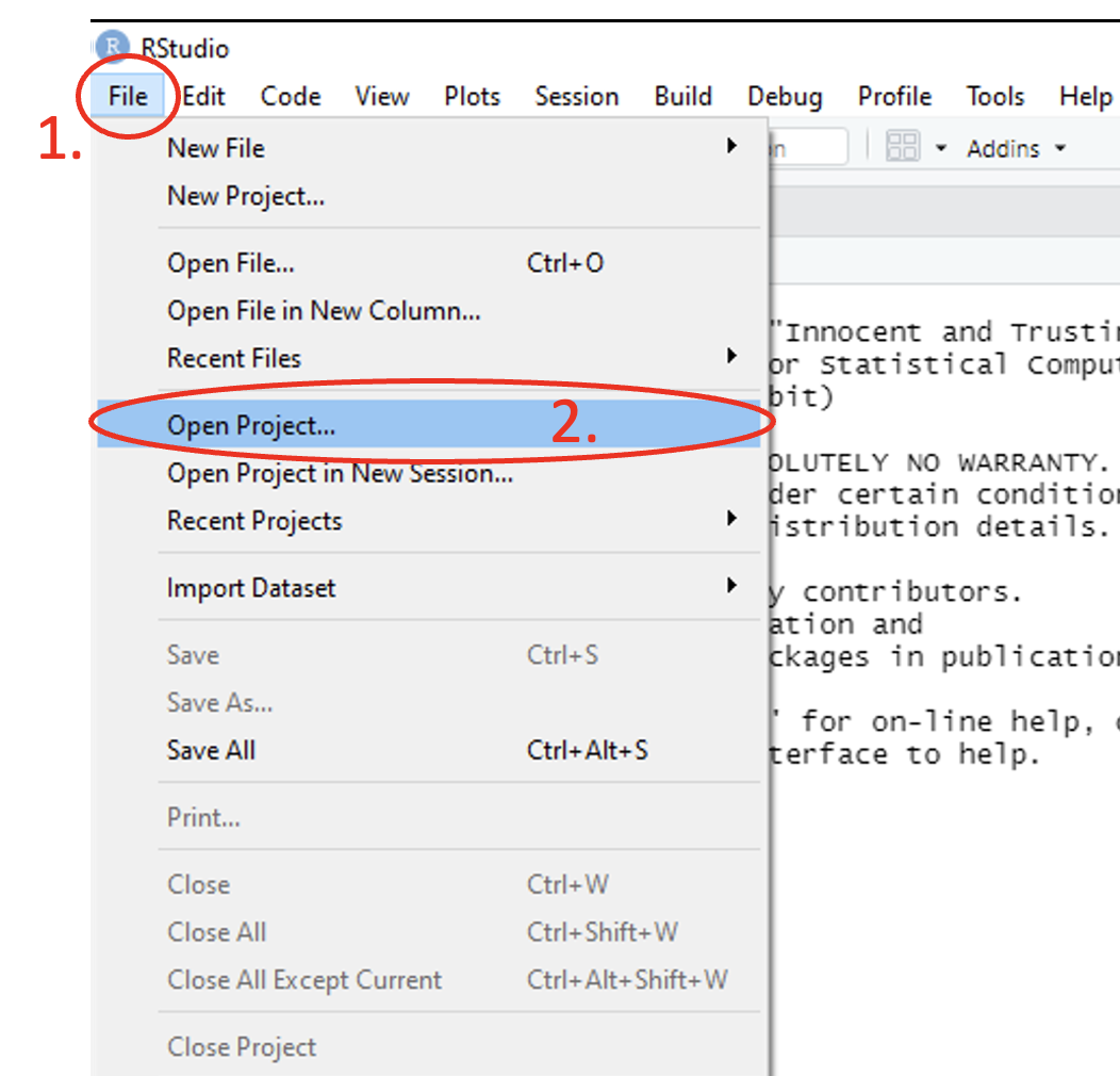
Figure 1.16: Annotated RStudio GUI: Open project

To save an R project, the same method is used as for R scripts, using the main toolbar and following the path File > Save As and navigate to the desired location in the pop-up file directory window and name the project To save updated versions of the project, use the main toolbar and follow File > Save.

1.1.3 Getting help in R

There are inbuilt facilities which provide information to help about any specific command or package in R.

The first method to get help in R is to run lines of code. For example, to get information about ‘mean’, run any of the following

help(mean): displays help in pane 3
?mean: displays help in pane 3
help.start(mean): displays help as html
??mean: displays help as html

Alternatively, use the toolbar of pane 3, navigate to the Help tab and use the search bar to look for the command.

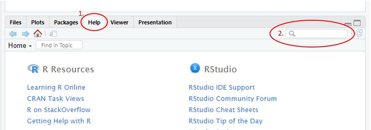
Figure 1.17: Annotated RStudio GUI: Help files

The help files for R functions and commands contain information on the following sections:

Description: A brief description on what the function(s) does and its usage
Usage: How to use the function(s) with what arguments need to be supplied and any default values of arguments
Arguments: Explanation on what the arguments are
Details: More in-depth information on the background of the function(s)
Value: Values that the function(s) returns
Source: What the function(s) is based on
References: Bibliography used for creating function(s)
See Also: Links to similar functions that may be of use
Examples: Examples on how to use the function(s)

If the information provided in the help files is insufficient, Stack Overflow is a great website where individuals can ask and answer questions. There are over 300,000 questions already asked on there so it is likely that the answer to your question has already been asked.

For some aspects of R, there are ‘Cheat Sheets’ available, posters which provide the essential, key information on the topic. To access this help, use the main toolbar and follow Help > Cheat Sheets > and select the file which matches your needs best. If the cheat sheet you require is not provided in the list, more options can be found by selecting Browse Cheat Sheets….

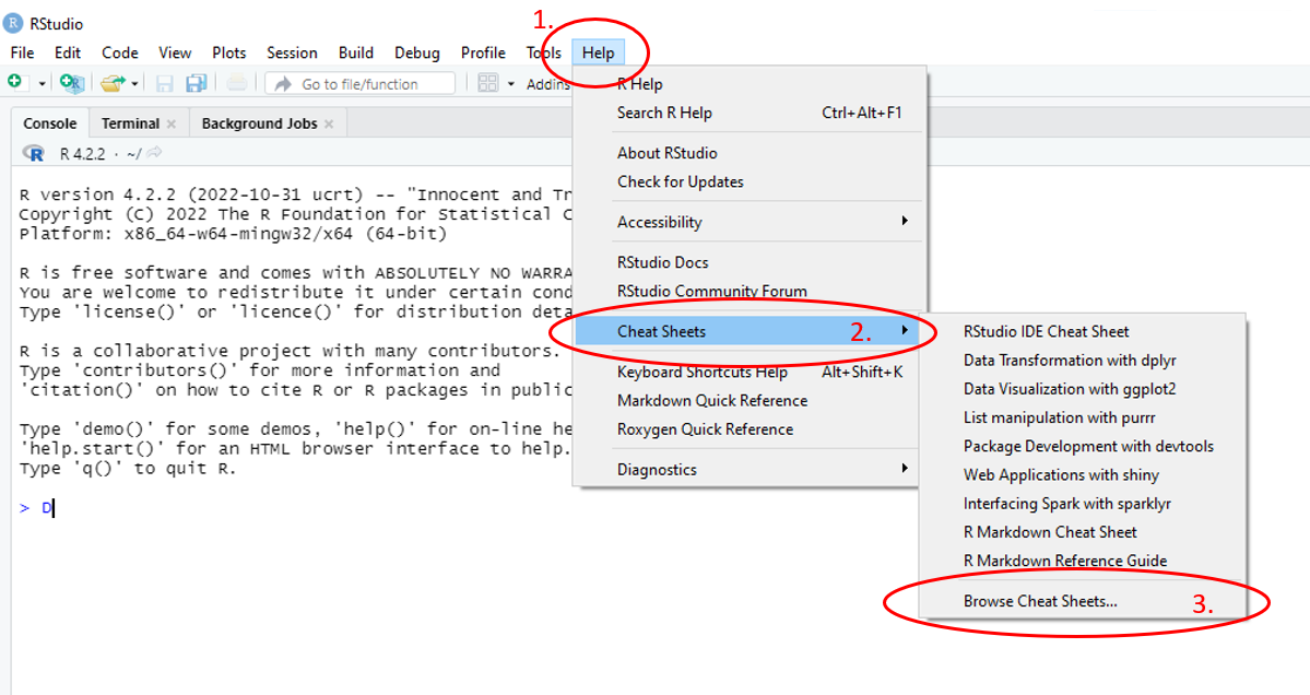
Figure 1.18: Annotated RStudio GUI: Help files

1.1.4 R coding best practices

1.1.4.1 Commenting

Including comments describing the code is good practice as it ensures that the code can be understood by both yourself in the future and others that the code is shared with. Comments can be added into the code by using the hash key, #, and stops the line being commented from running with the rest of the code.

#adding a comment with a hash tag ensures that yourself and others can understand
#the code quickly if returned to after some time.
X <- c(2, 3, 5, 7, 11, 13, 17, 19, 23, 29) #X contains prime numbers in order

Additionally, the hash can be used to create sections within scripts. To create a section, use at least 3 in a row without spaces in between (###). This is good practice for keeping your scripts organised.

1.1.4.2 Naming conventions

It is not only important to ensure anything in your code that is assigned a name is clear and identifiable, but also that the name chosen does not conflict with something that already has assignment by R (for example, c is already assigned to a function in R, used for combining values into vectors or lists). Some names are reserved by R, such as the names of existing functions. These names should not be used as your code will overwrite the existing code and the functions/values will no longer work.

To ensure that you are not assigning names that are not already taken, you can run the desired name and if it returns any code that you did not write, then R has already reserved that name. However, if it returns an error message, then the name is available for you to use.

#check if the name "abs" is available 
abs #"abs" is not available as it returns code for an existing function

## function (x)  .Primitive("abs")

#check if "absolute" is available instead
absolute #returns error message, "absolute" is free to use

## Error: object 'absolute' not found

#"c" is also not available 
c

## function (...)  .Primitive("c")

#"pi" is also not available 
pi

## [1] 3.141593

1.1.4.3 Spacing

R ignores spaces provided that they are not in the middle of a command name or operator. As a result, R treats the following as identical lines of code.

x<-1+2+3
x <- 1+2+3
x <- 1 + 2 + 3
x    <-    1   +     2     +   3

However, if you include the space in the middle of the operator, R will not return the result, but FALSE instead.

x < - 1 + 2 + 3

## [1] FALSE

R also ignores indentations at the start of a line, so spaces at the start of a line of code will appear the same as if there are no spaces. This is different to Python.

1.1.4.4 Punctuation

If you are putting different R commands on different lines, then there is no need for punctuation. However, if you are putting multiple R commands on the same line, then each command needs to be separated by a semicolon.

#separate each R command with a semicolon 
2*3; 4+5; 1-6

## [1] 6

## [1] 9

## [1] -5

1.2 Data types and key components

There are six common data types:

Boolean: logical statements e.g. TRUE, FALSE, T, F
Character: letters or non-numbers e.g. “alphabets”, “names”, …
Factor: non-numbers (characters) with levels, both ordered and unordered, with a predefined, finite number of values e.g. marital status field only allowing the options of: “single”, “separated”, “married”, “widowed/widower” or “divorced”
Integer: whole numbers e.g. 1L, 2L, 100L, …
Numeric: 1 and any number with decimals e.g. 1, 1.5, 8.9, …
Complex: complex numbers with real and imaginary parts e.g. 3+4i, 1-I, …

To check the data type in R, use the class() function.

There are three key components in R:

Objects: used to store values
Functions: allow for manipulations on objects to be performed
Operators: used to create interactions between objects or between an object and a function

1.2.1 Basic operations in R

1.2.1.1 Arithmetic operators


Operator	Description
`+`	addition
`-`	subtraction
`*`	multiplication
`/`	division
`^` or `**`	exponentiation
`%%`	modulus of a number
`%/%`	integer division
`%*%`	matrix multiplication

1.2.1.2 Logical operators


Operator	Description
`<`	less than
`<=`	less than or equal to
`>`	greater than
`>=`	greater than or equal to
`==`	exactly equal to
`!=`	not equal to
`!x`	not x
`&`	and
`\|`	or
`isTRUE(x)`	test if X is TRUE

1.2.1.3 Other operators


Operator	Description
`#`	commenting (do not run line)
`$`	extract value
`<-`	assign value to object
`=`	equals or assign value to object
`~`	assign variable to another

1.3 Key functions in R

Functions are always indicated with a name followed by (), and anything inside the parentheses is an argument, or option that is passed. Some arguments have a default value, meaning that if no value for that argument is given in the code, the default value will be used.

The following table contains some of the more commonly used functions that are available in base R, with a description of what they are used for. Examples on how to use many of these functions are seen later in the module.


Function	Description
`log()`	logarithm
`exp()`	exponential
`abs()`	absolute value
`seq()`	sequence of values
`sqrt()`	square root
`sd()`	standard deviation
`var()`	variance
`median()`	median
`mean()`	mean
`quantile()`	quantiles
`sum()`	add all elements together
`diff()`	difference
`min()`	minimum value/ element
`max()`	maximum value/ element
`range()`	gives smallest & largest numbers
`table()`	tabulation
`length()`	length of the vector
`summary()`	summarise the entire vector
`c()`	combine values into list or vector
`cbind()`	combine vectors, matrices or data frame by column
`rbind()`	combine vectors, matrices or data frame by row
`which()`	gives the TRUE indices of a logical object
`round()`	rounds the input to the specified accuracy
`paste()`	link vectors after converting to characters
`paste0()`	pastes everything as given
`cat()`	converts arguments to character strings
`print()`	outputs the object(s) given

Exercise: Which of the following will give a different output from the other 3? Hint: Look at the help file for the log() function.

log(x=6, base=4)
log(4, 6)
log(base=4, x=6)
log(6, 4)

1.4 Data structures

There are five data structures:

Vector: one dimensional where all elements must be of the same type, either numeric, character or factor
Matrix: two dimensional where data elements of the same data type are stored in rows and columns
Array: a data structure that contains multiple matrices where the elements are arranged sequentially
Data frame: two dimensional and can contain vectors of different data structures and can combine different variables
List: a flexible data structure that can contain all other data structures

1.4.1 Vectors

A vector can be a sequence of numbers, characters, logical, complex or a combination, and can be created in numerous ways.

One way of creating a vector is to use the function c() which combines the values input as arguments into a vector, providing that each value is separated with a comma.

#vector which contains the numbers 1, 2, 5, 3 and 7 in that order
c(1,2,5,3,7)

## [1] 1 2 5 3 7

If creating a vector that is a string of characters, it is imperative that each character is separated is enclosed by either ' or ".

Regions <- c("Northern", "Northeastern",
             "Western", "Central", "Eastern",
             "Southern")
Regions

## [1] "Northern"     "Northeastern" "Western"      "Central"      "Eastern"      "Southern"

A vector can be created to contain a combination of both numbers as strings.

mixed_vec <- c(4, "oranges", 5, "apples", 12, "carrots")
mixed_vec

## [1] "4"       "oranges" "5"       "apples"  "12"      "carrots"

Factors are related to vectors, and in R, factors are stored as integer vectors, where there are a finite number of categories and each level (or label) is a character. These can be created with the factor() function, inputting the vector you wish to convert to a factor as the argument.

#create factor for marital status
marital_status <- factor(c("single", "separated", "married", "widowed/widower",
                           "divorced", "married", "widowed/widower", "single",
                           "single", "married"))

#transform Regions to factor
Regions_fac <- factor(Regions)

To access the levels of the factor, you can either just print the variable itself or use the levels() function, inputting the factor variable as the argument.

#marital status levels
marital_status

##  [1] single          separated       married         widowed/widower divorced        married        
##  [7] widowed/widower single          single          married        
## Levels: divorced married separated single widowed/widower

#Regions levels
levels(Regions_fac)

## [1] "Central"      "Eastern"      "Northeastern" "Northern"     "Southern"     "Western"

The structure of the factor can be accessed with the str() function, where the output shows the different levels and indicates which level each of the elements of the variable are.

#structure of marital status
str(marital_status)

##  Factor w/ 5 levels "divorced","married",..: 4 3 2 5 1 2 5 4 4 2

Note: the data.frame() function explored later in this module automatically converts character vectors into factors if the argument stringsAsFactors=FALSE is not passed.

Another way to create a vector is to use a colon : which generates a regular sequence. a:b creates a sequence of numbers from a to b in increments/steps of either +1 or -1.

#vector of a sequence from 1 to 10, going up in increments of 1
1:10

##  [1]  1  2  3  4  5  6  7  8  9 10

#vector of a sequence from 20 to 10, going down in increments of 1 
20:10

##  [1] 20 19 18 17 16 15 14 13 12 11 10

#'a' and 'b' do not need to be integers:
#vector of a sequence from 5.5 to 15.5, going up in increments of 1
5.5:15.5

##  [1]  5.5  6.5  7.5  8.5  9.5 10.5 11.5 12.5 13.5 14.5 15.5

Also to create a vector, the function seq() in R can be used, with the following arguments:

from: the starting value (default=1)
to: the end value (default=1)
by: a numeric value indicating the size of each increment/step (default= (to-from)/(length.out-1))
length.out: a non-negative numeric value indicating the desired length of the sequence

#vector of a sequence from 1 to 50, going up in increments of 2
seq(from = 1, to = 51, by = 2)

##  [1]  1  3  5  7  9 11 13 15 17 19 21 23 25 27 29 31 33 35 37 39 41 43 45 47 49 51

#vector of a sequence from 1 to 50, with the sequence of length 20
seq(from = 1, to = 50, length.out = 20)

##  [1]  1.000000  3.578947  6.157895  8.736842 11.315789 13.894737 16.473684 19.052632 21.631579 24.210526
## [11] 26.789474 29.368421 31.947368 34.526316 37.105263 39.684211 42.263158 44.842105 47.421053 50.000000

The function rep() which replicates the value(s) input can also be used to create a vector in R, using the following arguments:

x: a number, vector or a factor which you want to replicate
times: a non-negative integer or integer-valued vector giving the number of times to repeat x
each: a non-negative integer giving the number of times to repeat each element in x in order/consecutively
length.out: a non-negative integer to give the value of the desired length of the vector

#vector of 1s repeated 10 times
rep(x = 1, times = 10)

##  [1] 1 1 1 1 1 1 1 1 1 1

#vector of a sequence from 1 to 10, going up in increments of 1, repeated twice
rep(x = 1:10, times = 2)

##  [1]  1  2  3  4  5  6  7  8  9 10  1  2  3  4  5  6  7  8  9 10

#vector of a sequence from 1 to 10, going up in increments of 1, where each 
#element is repeated twice consecutively
rep(x = 1:10, each = 2)

##  [1]  1  1  2  2  3  3  4  4  5  5  6  6  7  7  8  8  9  9 10 10

#vector of a sequence from 1 to 10, going up in increments of 1, repeated until
#the length of the vector is 15
rep(x = 1:10, length.out = 15)

##  [1]  1  2  3  4  5  6  7  8  9 10  1  2  3  4  5

Exercise: Create a vector that goes from 5 to 25 by increments of 1.

A combination of the different vector construction methods can be used at once, for example, the combine function c() can be used within the other functions and can also be used to combine existing vectors.

vec1 <- seq(from = 10, to = 100, by = 10) 
vec2 <- rep(x = 15:10, each = 2)
#combine vectors vec1 and vec2
vec3 <- c(vec1, vec2) 
vec3

##  [1]  10  20  30  40  50  60  70  80  90 100  15  15  14  14  13  13  12  12  11  11  10  10

Exercise: Create another vector that goes from 5 to 25 by increments of 1, but using a different method. Call this vector V1

Elements from vectors can be indexed (selected) using square brackets [].

#extract the first (1st) element from vec1
vec1[1]

## [1] 10

#extract the first (1st), fourth (4th) and sixth (6th) element from vec2
vec2[c(1, 4, 6)]

## [1] 15 14 13

#show all elements of vec2 except the 4th and 5th elements
vec2[-c(4, 5)]

##  [1] 15 15 14 13 12 12 11 11 10 10

#element-wise calculations: multiply the third (3rd) element from vec3 by the 
#fourth (4th) element of vec2
vec3[3]*vec2[4]

## [1] 420

Exercise: Extract the 5th element of V1.

Through indexing elements from vectors, elements within vectors can be updated.

mixed_vec

## [1] "4"       "oranges" "5"       "apples"  "12"      "carrots"

#update the first (1st) element of mixed_vec from 4 to 6
mixed_vec[1] <- 6 
#update the second (2nd) and fourth (4th) elements of mixed_vec from oranges 
#and apples to lemons and bananas
mixed_vec[c(2, 4)] <- c("lemons", "bananas") 
mixed_vec

## [1] "6"       "lemons"  "5"       "bananas" "12"      "carrots"

Exercise: Remove the 7th element from the vector V1 and call this new vector V2.

Vectors can be summarised, inputting the vector into functions different functions.

#find the length of vec1
length(vec1)

## [1] 10

#sum the elements of vec2
sum(vec2)

## [1] 150

#find the mean of the elements in vec3
mean(vec3)

## [1] 31.81818

#create a vector
vec4 <- c(12, 3, -1, 239, 84 ) 
#find the mean of the elements in vec4
mean(vec4)

## [1] 67.4

#round the mean of vec4 to the nearest whole number
round(x = mean(vec4), digits = 0)

## [1] 67

Logical operators can be used with vectors to return TRUE or FALSE for each element depending on the conditions given.

#return TRUE for elements which are both greater than 10 and less than 100, and 
#FALSE if both conditions are not met
vec4 > 10 & vec4 < 100

## [1]  TRUE FALSE FALSE FALSE  TRUE

Indexing used with logical vectors returns the elements in the vector which meet the conditions given.

#both conditions must be true, greater than 10 AND less than 100
vec4[vec4 > 10 & vec4 < 100]

## [1] 12 84

#either condition can be true, greater than 100 OR less than 0
vec4[vec4 > 100 | vec4 < 0]

## [1]  -1 239

The function which() can be used in conjunction with logical operators to return the index/indices of the element(s) which meet the conditions given, rather than the logical statements or values.

#gives the indices of the elements in vec4 which are greater than 10
which(vec4 > 10)

## [1] 1 4 5

Extensions of the which() function are which.min() and which.max() which respectively give the indices of the elements with the minimum value and the maximum value.

#gives index of the element in vec4 which has the smallest value
which.min(vec4)

## [1] 3

#gives index of the element in vec4 which has the largest value
which.max(vec4)

## [1] 4

Exercise: How many elements in your vector, V1, are greater than 11?

1.4.2 Matrices

Used for data storage and often faster to work with than a data frame.

Create a matrix using the function matrix() in R, with the following arguments:

data: the data that you want to include in the matrix
nrow: the number of rows you want the matrix to have
ncol: the number of columns you want the matrix to have
byrow: logical, if FALSE (the default), the matrix fills by columns, if TRUE, the matrix fills by row
dimnames: (optional, NULL by default) input a list of length 2, containing the row and column names respectively

#example of creating a 4x4 matrix:
mat <- matrix(data = seq(1, 16), nrow = 4, ncol = 4, byrow = TRUE)
mat

##      [,1] [,2] [,3] [,4]
## [1,]    1    2    3    4
## [2,]    5    6    7    8
## [3,]    9   10   11   12
## [4,]   13   14   15   16

#combine two matrices by column:
matrix1 <- matrix(data = 1, nrow = 2, ncol = 2)
matrix2 <- matrix(data = 2, nrow = 2, ncol = 2)

#returns a 2x4 matrix
cbind(matrix1, matrix2)

##      [,1] [,2] [,3] [,4]
## [1,]    1    1    2    2
## [2,]    1    1    2    2

Matrices can also be created through combining multiple vectors.

#create two vectors of the same length
vec_mat_a <- 1:10
vec_mat_b <- 11:20
#use rbind to create a 2x10 matrix
vec_mat1 <- rbind(vec_mat_a, vec_mat_b)
vec_mat1

##           [,1] [,2] [,3] [,4] [,5] [,6] [,7] [,8] [,9] [,10]
## vec_mat_a    1    2    3    4    5    6    7    8    9    10
## vec_mat_b   11   12   13   14   15   16   17   18   19    20

#use cbind to create a 10x2 matrix
vec_mat2 <- cbind(vec_mat_a, vec_mat_b)
vec_mat2

##       vec_mat_a vec_mat_b
##  [1,]         1        11
##  [2,]         2        12
##  [3,]         3        13
##  [4,]         4        14
##  [5,]         5        15
##  [6,]         6        16
##  [7,]         7        17
##  [8,]         8        18
##  [9,]         9        19
## [10,]        10        20

Exercise: Create a matrix that contains the sequence of numbers from 1 to 16, going up in increments of 1. Let the matrix have 4 rows and have the matrix elements fill by row. Call this matrix M1.

To check the dimensions of a matrix, you can use the function dim().

dim(vec_mat1)

## [1]  2 10

dim(vec_mat2)

## [1] 10  2

Using square brackets [,] you can take subsets of matrices, the first element in the square bracket corresponds to the row indexing and the second element corresponds to the column indexing, [row, column].

# a vector of all the first row elements of the matrix 
mat[1,]

## [1] 1 2 3 4

# a vector of all the first column elements of the matrix 
mat[,1]

## [1]  1  5  9 13

You can subset multiple rows and multiple columns by indexing using vectors.

#a matrix containing the first and second rows of the matrix
mat[c(1,2),]

##      [,1] [,2] [,3] [,4]
## [1,]    1    2    3    4
## [2,]    5    6    7    8

#a matrix containing the third and fourth columns of the matrix
mat[,c(3,4)]

##      [,1] [,2]
## [1,]    3    4
## [2,]    7    8
## [3,]   11   12
## [4,]   15   16

Both rows and columns can be indexed for selecting either a single element from a matrix or indexing a selection of rows and columns only.

#a single element from the 4th row and the 4th column of the matrix
mat[4,4]

## [1] 16

#a matrix containing elements present in the first and second rows AND the 
#third and fourth columns
mat[c(1,2), c(3,4)]

##      [,1] [,2]
## [1,]    3    4
## [2,]    7    8

Exercise: Extract the 3rd and 4th rows and the 1st and 2nd columns of your matrix, M1. Call this matrix M2.

As with vectors, through indexing, elements of the matrix can be updated.

citrus_mat <- matrix(data = c("oranges", "lemons", "limes", "apples"), 
                     nrow = 2, ncol = 2, byrow = TRUE)
citrus_mat

##      [,1]      [,2]    
## [1,] "oranges" "lemons"
## [2,] "limes"   "apples"

#update the element in the second (2nd) row and the second (2nd) column to also
#be a citrus fruit
citrus_mat[2,2] <- "pomelo" 
citrus_mat

##      [,1]      [,2]    
## [1,] "oranges" "lemons"
## [2,] "limes"   "pomelo"

The functions rowSums() and colSums() are used to find the row sums and column sums respectively, returning a vector of the values.

#returns a vector of the row sums
rowSums(mat)

## [1] 10 26 42 58

#returns a vector of the column sums
colSums(mat)

## [1] 28 32 36 40

The apply() function can be used to obtain row or column summaries of a data matrix, with the following arguments:

X: the matrix you wish to summarise
MARGIN: a vector that indicates which subscripts to apply the function to. For example, 1 indicates all rows, 2 indicates all columns and c(1,2) indicates rows and columns
FUN: the function that is to be applied to the data
simplify: logical, if TRUE (the default), results will be simplified if possible

#calculates the column sums of the matrix
apply(mat, 2, sum)

## [1] 28 32 36 40

#calculates the row means of the matrix
apply(mat, 1, mean)

## [1]  2.5  6.5 10.5 14.5

Exercise: Find the row sums of the matrix M2.

To multiply two matrices together, the operator %*% can be used, providing that the two matrices conform (the number of columns of one matrix must be equal to the number of rows on the other one).

#multiply the two 2x2 matrices together
matrix1%*%matrix2

##      [,1] [,2]
## [1,]    4    4
## [2,]    4    4

1.4.3 Arrays

An array contains one or more matrices.

Create an array using the function array() in R, with the following arguments:

data: a vector containing data to fill the array
dim: an integer vector of length one or more giving the dimensions of the array
dimnames: a list with one component for each dimension of the array

#an array of 3, 3x3 matrices
array1 <- array(c(round(seq(1,36, length=9)), 
             round(seq(10,30, length=9)), 
             round(seq(40,200, length=9))),
           dim=c(nrow=3,ncol=3, 3))

Arrays can be subset in the same way as matrices, using square brackets, except with an extra comma to indicate which of the matrices in the array is to be indexed.

#subsets the first matrix in the array
array1[,,1]

##      [,1] [,2] [,3]
## [1,]    1   14   27
## [2,]    5   18   32
## [3,]   10   23   36

1.4.4 Data frames

A data frame is a two-dimensional, tabular data type which can store multiple data types in R. It is also the most widely used data format as it can combine different types of variables.

You can create a data frame by using the function data.frame(), combining collections of variables.

For an example, a data frame can be constructed by creating some dummy/fake data:

##--Create some dummy or fake data
#paste0 function pastes everything together, returns region1, ..., region6
regions = paste0("region", 1:6) 

tot_pop <- c(1000000, 920000, 2050000, 3100000, 1535000, 743000) 
tot_hh <- c(200505, 124000, 882012,1051200, 452000, 79000) 
male_prop <- c(0.55, 0.49, 0.45, 0.58, 0.56, 0.55)
male_pop <- tot_pop*male_prop
female_pop <- tot_pop - male_pop

and then using the function data.frame(), using the variables created above as the arguments:

data_frame1 <- data.frame(Region = regions,Tot_pop = tot_pop,Tot_hh = tot_hh, 
                          Male_pop = male_pop, Female_pop = female_pop)
data_frame1

##    Region Tot_pop  Tot_hh Male_pop Female_pop
## 1 region1 1000000  200505   550000     450000
## 2 region2  920000  124000   450800     469200
## 3 region3 2050000  882012   922500    1127500
## 4 region4 3100000 1051200  1798000    1302000
## 5 region5 1535000  452000   859600     675400
## 6 region6  743000   79000   408650     334350

1.4.5 List

A list is a vector where each element itself is an object. Informally, it can be described as a ‘bag’ that contains data of different forms, types and dimensions, including other lists.

Create a list using the function list() in R, for example:

#create a list using the variables, matrices and arrays from above
list1 <- list(Admin = Regions, matrix = mat, array = array1) 
list1

## $Admin
## [1] "Northern"     "Northeastern" "Western"      "Central"      "Eastern"      "Southern"    
## 
## $matrix
##      [,1] [,2] [,3] [,4]
## [1,]    1    2    3    4
## [2,]    5    6    7    8
## [3,]    9   10   11   12
## [4,]   13   14   15   16
## 
## $array
## , , 1
## 
##      [,1] [,2] [,3]
## [1,]    1   14   27
## [2,]    5   18   32
## [3,]   10   23   36
## 
## , , 2
## 
##      [,1] [,2] [,3]
## [1,]   10   18   25
## [2,]   12   20   28
## [3,]   15   22   30
## 
## , , 3
## 
##      [,1] [,2] [,3]
## [1,]   40  100  160
## [2,]   60  120  180
## [3,]   80  140  200

Data can be retrieved from a list using the dollar sign $, and subset the retrieved data in the same way as without lists.

list1$Admin

## [1] "Northern"     "Northeastern" "Western"      "Central"      "Eastern"      "Southern"

list1$array1[,,2]

## NULL

Logical operators can be used to subset data within a list.

#returns TRUE for element(s) which are greater than 20 and FALSE otherwise
list1$vector>20

## logical(0)

#returns TRUE for element(s) which are exactly equal to 10 and FALSE otherwise 
list1$matrix==10

##       [,1]  [,2]  [,3]  [,4]
## [1,] FALSE FALSE FALSE FALSE
## [2,] FALSE FALSE FALSE FALSE
## [3,] FALSE  TRUE FALSE FALSE
## [4,] FALSE FALSE FALSE FALSE

Using the dollar sign, $, new variables can be added to a list.

list1$vector <- vec3
list1

## $Admin
## [1] "Northern"     "Northeastern" "Western"      "Central"      "Eastern"      "Southern"    
## 
## $matrix
##      [,1] [,2] [,3] [,4]
## [1,]    1    2    3    4
## [2,]    5    6    7    8
## [3,]    9   10   11   12
## [4,]   13   14   15   16
## 
## $array
## , , 1
## 
##      [,1] [,2] [,3]
## [1,]    1   14   27
## [2,]    5   18   32
## [3,]   10   23   36
## 
## , , 2
## 
##      [,1] [,2] [,3]
## [1,]   10   18   25
## [2,]   12   20   28
## [3,]   15   22   30
## 
## , , 3
## 
##      [,1] [,2] [,3]
## [1,]   40  100  160
## [2,]   60  120  180
## [3,]   80  140  200
## 
## 
## $vector
##  [1]  10  20  30  40  50  60  70  80  90 100  15  15  14  14  13  13  12  12  11  11  10  10

Lists can be also be created to demonstrate different levels, for example, age ranges.

Age  <- list(Infant = "0-59 months",
            Child = "5 - 12 years",
            Teen = "13 - 17 years", 
            Adult = "18+")
Age

## $Infant
## [1] "0-59 months"
## 
## $Child
## [1] "5 - 12 years"
## 
## $Teen
## [1] "13 - 17 years"
## 
## $Adult
## [1] "18+"

Lists can be ‘flattened’ using the function unlist(), which simplifies the list into a vector which contains the same elements.

Age_unlist <- unlist(Age)
Age_unlist

##          Infant           Child            Teen           Adult 
##   "0-59 months"  "5 - 12 years" "13 - 17 years"           "18+"

1.5 End of module exercises

1. Use R to find the value of the square root of 25. ($\sqrt(25)$) Hint: Look at the help file for the function sqrt().

2. Use R to find the value of the exponential of $6\times 14 -3$. ($\exp(6\times 14-3)$)

3. Use R to find the value of the absolute value of $7\times 3 - 4\times 9 - 30$. ($|7\times 3 - 4\times 9 - 30|$)

4. Use R to find the value of $\frac{73-42}{3}+2\times\left(\frac{36}{4}-17\right)$. Give your answer to 2 decimal places.

5. How many elements does the following vector have?

seq(from = 0, to = 100, by = 3.14)

6. Look at the help file for the function rnorm() and use this function to generate 100 random numbers with mean 10 and standard deviation 5.

WorldPop Population Modelling Training Manual, Vol. I