Basic building footprint calculations
November 10, 2021
Source:vignettes/footsteps.Rmd
footsteps.RmdThe foot package was developed by WorldPop at the University of Southampton (www.worldpop.org) to provide a set of consistent and flexible tools for processing 2D vector representations of buildings (e.g. “footprints”) and calculating urban morphology measurements. The functionality includes basic geometry and morphology characteristics, distance and clustering metrics. These calculations are supported with helper functions for spatial intersections and tiled reading/writing of data.
This vignette will demonstrate some of the core functionality in the package, including:
- The available measurements and summary statistics
- How to define different types of spatial zones for area-level summaries
- Calculating multiple summary metrics for a set of spatial areas
- Example workflows to produce outputs using
foot::calculate_footstats().
To demonstrate the package, this vignette will use a supplied sample of building footprint polygons produced by Microsoft Bing Maps (Source) from an area in Kampala, Uganda. These footprints have been reprocessed into a spatial data format which can be read with sf.
Load the sample dataset
data("kampala", package = "foot")

buildings <- kampala$buildings
adminzones <- kampala$adminZones
clusters <- kampala$clusters
The sample dataset is a list of four named objects:
- “buildings” - polygons of building footprints in
sfformat. Contains 8480 records. - “mastergrid” - geoTiff
RasterLayeraligned to WorldPop datalayers. This will be used as a template for producing other gridded outputs - “adminZones” - 34 polygons in
sfformat for zonal statistics - “clusters” - 10 small polygons in
sfformat for sample sites
Note that the adminZones and cluster boundaries are purely artificial and were created for demonstration purposes only.
For more information, see ?kampala.
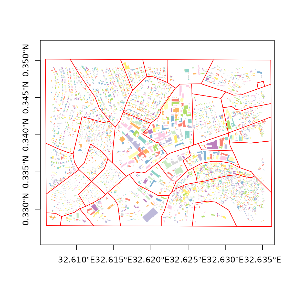
Sample buildings and zones in Kampala
Calculations with foot
The core functions of foot are provided by calculate_footstats(). The operations include: 1) calculating geometry measures for each footprint, 2) summarising one or more geometry measures of footprints within zones. The simplest usage involves supplying a set of building footprint polygons and the desired characteristics to calculate. All operations return the same format - a data.table, optionally with a column for the index and the named column for the summarised footprint metric(s).
# the area and perimeter of each building footprint
built_area <- calculate_footstats(buildings, what = list("area", "perimeter"))
#> Selecting metrics
#> Setting control values.
#> Pre-calculating areas
#> Pre-calculating perimeters
#> No summary functions found, returning metrics.

head(built_area)
#>               area    perimeter
#> 1:  22.10707 [m^2] 19.26045 [m]
#> 2: 221.37976 [m^2] 67.95023 [m]
#> 3:  39.13247 [m^2] 25.37269 [m]
#> 4: 388.48091 [m^2] 98.55654 [m]
#> 5: 351.14738 [m^2] 82.22555 [m]
#> 6: 164.74579 [m^2] 55.87172 [m]
To summarise the footprint characteristics over all building polygons, the name of a summary function, or a list of multiple functions can be supplied.
# the average and standard deviation of all building areas
calculate_footstats(buildings, what = "area", how = list("mean", "sd"))
#> Selecting metrics
#> Setting control values.
#> Pre-calculating areas
#>
#> Calculating  2  metrics ...
#>    area mean
#>    area sd
#> Finished calculating metrics.
#>    zoneID      area_mean  area_sd
#> 1:      1 264.3684 [m^2] 718.4919
Available metrics and summary measures
Currently implemented are measures for:
- building presence
- area
- perimeter
- nearest neighbour distance
- angle of rotation
- compactness and shape
- length-width ratio
A table of metrics and other packaged summary function names available for each is available using list_fs(). The results of this function provide “cols” and “funs” which can be passed as what and how arguments, respectively, to calculate_footstats.
# get all available built-in functions for perimeter calculations
argsList <- list_fs(what = "perimeter")

calculate_footstats(buildings, what = argsList$cols, how = argsList$funs)
#> Selecting metrics
#> Setting control values.
#> Pre-calculating perimeters
#>
#> Calculating  8  metrics ...
#>    perimeter cv
#>    perimeter iqr
#>    perimeter max
#>    perimeter mean
#>    perimeter median
#>    perimeter min
#>    perimeter sd
#>    perimeter sum
#> Finished calculating metrics.
#>    zoneID perimeter_cv perimeter_iqr perimeter_max perimeter_mean
#> 1:      1    0.9396027      40.81674  1089.097 [m]   62.22027 [m]
#>    perimeter_median perimeter_min perimeter_sd perimeter_sum
#> 1:     46.68314 [m]  14.88332 [m]     58.46233  301146.1 [m]
With no other argument supplied, all the footprints are treated as coming from the same spatial zone for any summary function. A later section describes the process for identifying zones.
Additional characteristics and geometry measures
Whenever possible, foot makes use of generic functions within R. Most low-level geometry calculations rely on sf, geos, lwgeom and users need to have recent versions of these packages installed. There are other stand-alone functions within foot to support more complex or less-common measurements.
Nearest neighbour distances
Distances can be calculated between footprints, or between footprints and other spatial objects. The distances can be measured edge-to-edge (method = "poly") or the centroids of the building footprints can be used (method = "centroid").
# nearest distance for the first 10 buildings to any other building measured
# between polygon edges
fs_nndist(buildings[1:10, ], buildings, maxSearch = 200, unit = "m")
#> Units: [m]
#>  [1]  3.9782228  7.9372980  1.0249509 22.3497210  2.4816995 16.2608819
#>  [7]  0.9555975  1.8666478  2.6156498  2.3014386

# omitting argument 'Y' measures distance among the footprints supplied setting
# maxSearch=NULL removes the search restriction
fs_nndist(buildings[1:10, ], method = "centroid", maxSearch = NULL)
#> Units: [m]
#>  [1] 100.15489 100.15489  90.59004  90.59004 117.26008 117.26008 218.52524
#>  [8] 228.62489 218.52524 440.20521
Note that distance calculations are slower for polygons and for unprojected coordinate systems. The centroid-based calculations are faster. It is recommended that a maximum search radius is always used. Internally the calculations are done with a data.table to benefit from multi-threading capabilities.
Rotation angles
A less conventional geometric measure is derived from the rotated bounding rectangle. This is the rectangle enclosing a footprint polygon which has been rotated to minimise the area. In contrast, a “bounding box” for a polygon is always oriented along the x and y axes.
# To obtain the rotated rectangle as a spatial object
mbr <- fs_mbr(buildings[4502, ], returnShape = T)

plot(sf::st_geometry(buildings[4502, ]), col = "grey")
plot(mbr, border = "red", lwd = 2, add = T)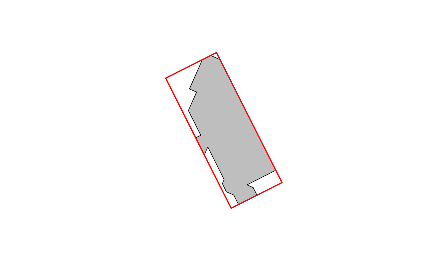
# Or obtain just the angle measure
fs_mbr(buildings[4502, ], returnShape = F)
#> [1] 153.0991
The angles can be summarised as an entropy measure and normalised to describe how much the angles of a set of structures depart from a regular grid pattern (available in calculate_footstats where how = "entropy").
Creating and supplying zone indices
Rather than treating all footprints features as belonging to a single summary zone, it’s more common to want to summarise metrics within smaller areas. There are several ways to supply information on the zones.
Index by vector
A vector of indices for the zones can be supplied to foot functions as a 1) column name within the footprints, 2) a standalone numeric vector of indices, or 3) a spatial polygons object to join to the building footprints. The length of a vector of indices must match the number of building polygons.
# create a vector of ten random zones
idx <- sample(1:10, nrow(buildings), replace = T)
buildings$id <- idx  # add it to the buildings object
table(buildings$id)  # splitting observations into 10 groups
#>
#>   1   2   3   4   5   6   7   8   9  10
#> 490 502 547 506 473 510 475 436 432 469

# 1. pass the index by name
colnames(buildings)
#> [1] "FID_1"    "geometry" "id"
calculate_footstats(buildings, "id", what = "area", how = "mean", verbose = FALSE)
#>     id      area_mean
#>  1:  1 277.3981 [m^2]
#>  2:  2 224.0173 [m^2]
#>  3:  3 253.2530 [m^2]
#>  4:  4 260.3614 [m^2]
#>  5:  5 298.4207 [m^2]
#>  6:  6 231.7565 [m^2]
#>  7:  7 289.4302 [m^2]
#>  8:  8 218.9365 [m^2]
#>  9:  9 317.8345 [m^2]
#> 10: 10 279.9572 [m^2]

# 2. pass the index as a standalone vector
calculate_footstats(buildings, idx, what = "settled", how = "count", verbose = FALSE)
#>     zoneID settled_count
#>  1:      1           490
#>  2:      2           502
#>  3:      3           547
#>  4:      4           506
#>  5:      5           473
#>  6:      6           510
#>  7:      7           475
#>  8:      8           436
#>  9:      9           432
#> 10:     10           469

# 3. pass a separate spatial object of zones
calculate_footstats(buildings, zone = adminzones, what = "angle", how = "entropy",
    verbose = FALSE)
#>     zoneID angle_entropy
#>  1:      1    0.57343067
#>  2:      2    0.11127610
#>  3:      3    0.41727642
#>  4:      4    0.17619017
#>  5:      5    0.42197650
#>  6:      6    0.49947882
#>  7:      7    0.82533100
#>  8:      8    0.44538996
#>  9:      9    0.07920041
#> 10:     10    0.38729360
#> 11:     11    0.22977920
#> 12:     12    0.46026280
#> 13:     13    0.97518024
#> 14:     14    0.21544105
#> 15:     15    0.10321490
#> 16:     16    0.16620845
#> 17:     17    0.13136813
#> 18:     18    0.05440004
#> 19:     19    0.05390193
#> 20:     20    0.05590684
#> 21:     21    0.21223559
#> 22:     22    0.43947190
#> 23:     23    0.08843299
#> 24:     24    0.07816555
#> 25:     25    0.69100714
#> 26:     26    0.10747520
#> 27:     27    0.10629896
#> 28:     29    0.13106462
#> 29:     30    0.26117524
#> 30:     31    0.60237738
#> 31:     32    0.16687157
#> 32:     33    0.70065801
#> 33:     34    0.04253442
#>     zoneID angle_entropy
Index by zone shapes
Rather than supplying a pre-calculated column or vector of zonal indices, buildings can be assigned a zone based on a spatial join. When the index is created in the building footprints, it will be named “zoneID” or a user-specified name.
# examine the other objects loaded from supplied data
head(adminzones)
#> Simple feature collection with 6 features and 1 field
#> Geometry type: POLYGON
#> Dimension:     XY
#> Bounding box:  xmin: 32.60589 ymin: 0.3277355 xmax: 32.62531 ymax: 0.3388665
#> Geodetic CRS:  WGS 84
#>   Id                       geometry
#> 1  1 POLYGON ((32.61231 0.327771...
#> 2  2 POLYGON ((32.61034 0.335317...
#> 3  3 POLYGON ((32.61592 0.327757...
#> 4  4 POLYGON ((32.6214 0.3277355...
#> 5  5 POLYGON ((32.62342 0.333760...
#> 6  6 POLYGON ((32.62498 0.335199...
head(clusters)
#> Simple feature collection with 6 features and 1 field
#> Geometry type: POLYGON
#> Dimension:     XY
#> Bounding box:  xmin: 32.60624 ymin: 0.3303863 xmax: 32.63375 ymax: 0.3472696
#> Geodetic CRS:  WGS 84
#>   Id                       geometry
#> 1  1 POLYGON ((32.6066 0.3398617...
#> 2  2 POLYGON ((32.61151 0.337602...
#> 3  3 POLYGON ((32.61028 0.331954...
#> 4  4 POLYGON ((32.61649 0.344649...
#> 5  5 POLYGON ((32.62552 0.345516...
#> 6  6 POLYGON ((32.63225 0.340927...

# Return a table of index values based on administrative zone polygons using
# the standalone function within `foot`
zID <- zonalIndex(buildings, adminzones, returnObject = F)
head(zID, 10)  # the xID column are row numbers to object X
#>      xID zoneID
#>  1:  463      1
#>  2:  531      1
#>  3:  848      1
#>  4: 1372      1
#>  5: 1504      1
#>  6: 1534      1
#>  7: 1859      1
#>  8: 1939      1
#>  9: 2121      1
#> 10: 2414      1

# Alternatively (and preferably), join zones to create a new footprint object A
# custom zone name can be used but must be specificed to the summary functions
zObj <- zonalIndex(buildings, clusters, zoneField = "Id", returnObject = T)
zObj
#> Simple feature collection with 348 features and 3 fields
#> Geometry type: POLYGON
#> Dimension:     XY
#> Bounding box:  xmin: 32.60631 ymin: 0.328119 xmax: 32.63543 ymax: 0.349785
#> Geodetic CRS:  WGS 84
#> First 10 features:
#>     FID_1 id Id                       geometry
#> 1   17706  1  1 POLYGON ((32.60662 0.339353...
#> 2   72387  1  1 POLYGON ((32.60769 0.338973...
#> 3   78504  1  1 POLYGON ((32.60703 0.338654...
#> 4  106647  1  1 POLYGON ((32.60793 0.339799...
#> 5  150833  1  1 POLYGON ((32.60712 0.338893...
#> 6  289245  1  1 POLYGON ((32.60788 0.339471...
#> 7   57187  2  1 POLYGON ((32.60827 0.338821...
#> 8   68588  2  1 POLYGON ((32.60787 0.338906...
#> 9  127999  2  1 POLYGON ((32.60707 0.339934...
#> 10 257296  2  1 POLYGON ((32.60692 0.339061...
When using a new spatial object which has been joined to its zones, remember to supply the name of the zone field to calculate_foostats.
# use the new object and zone field 'Id' in a summary calculation
colnames(zObj)
#> [1] "FID_1"    "id"       "Id"       "geometry"

zarea <- calculate_footstats(zObj, zone = "Id", what = "area", how = "mean", verbose = F)
clusters <- merge(clusters, zarea, by = "Id")
plot(sf::st_geometry(adminzones))
plot(clusters["area_mean"], add = T)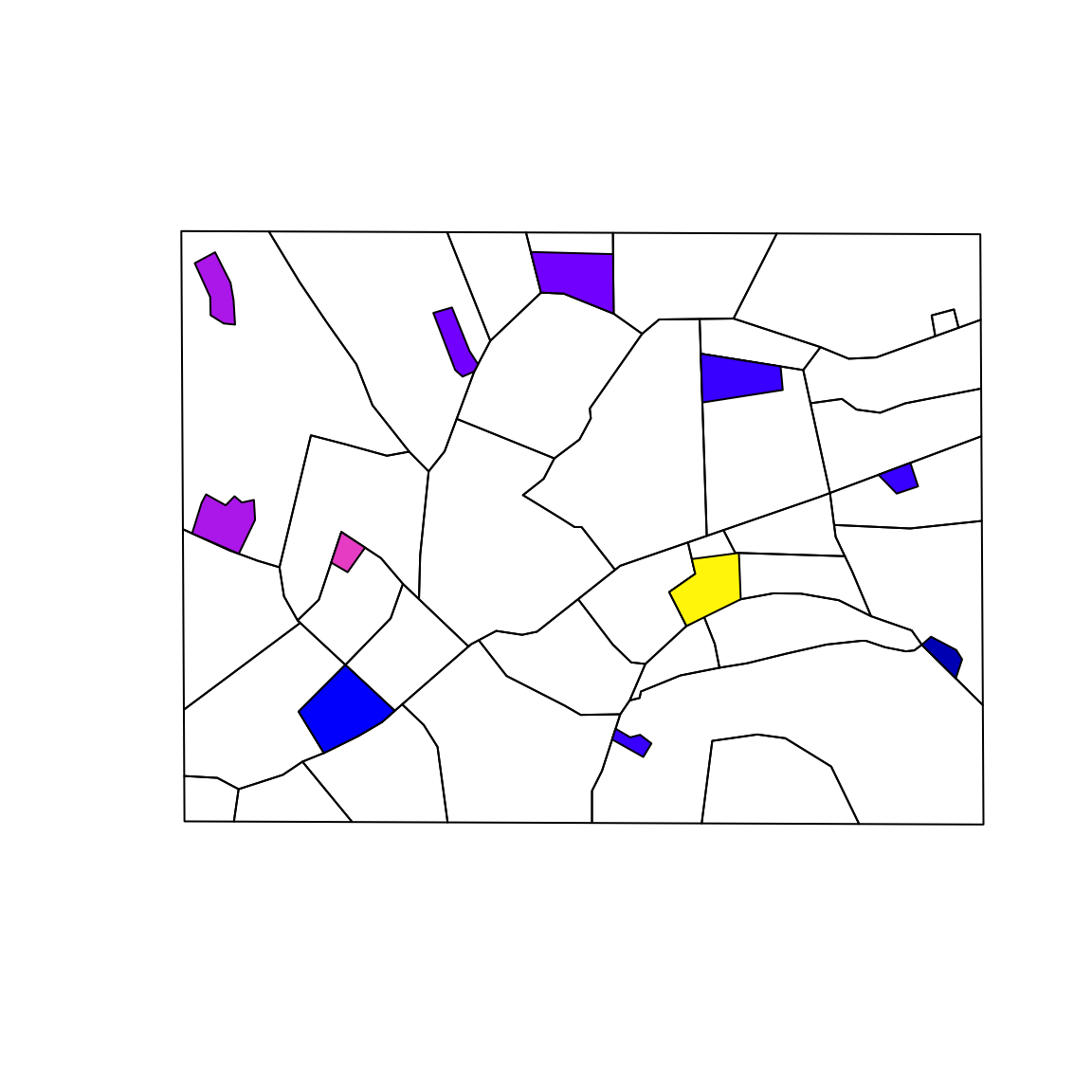
The zonalIndex function works by spatial intersection. This produces some (potentially useful) side effects that users need to be aware of. Specifically, note that if a building footprint intersects more than 1 zone it will be duplicated and associated to all intersecting zones.
The default behaviour (see method) is to assign a building to a zone based on its centroid.
# Note the selected structures extend beyond the cluster boundary
plot(sf::st_geometry(clusters)[[6]])
plot(sf::st_geometry(buildings), add = T)
plot(sf::st_geometry(zObj[zObj$Id == 6, ]), col = "red", add = T)
plot(sf::st_geometry(sf::st_centroid(zObj[zObj$Id == 6, ])), pch = 16, add = T)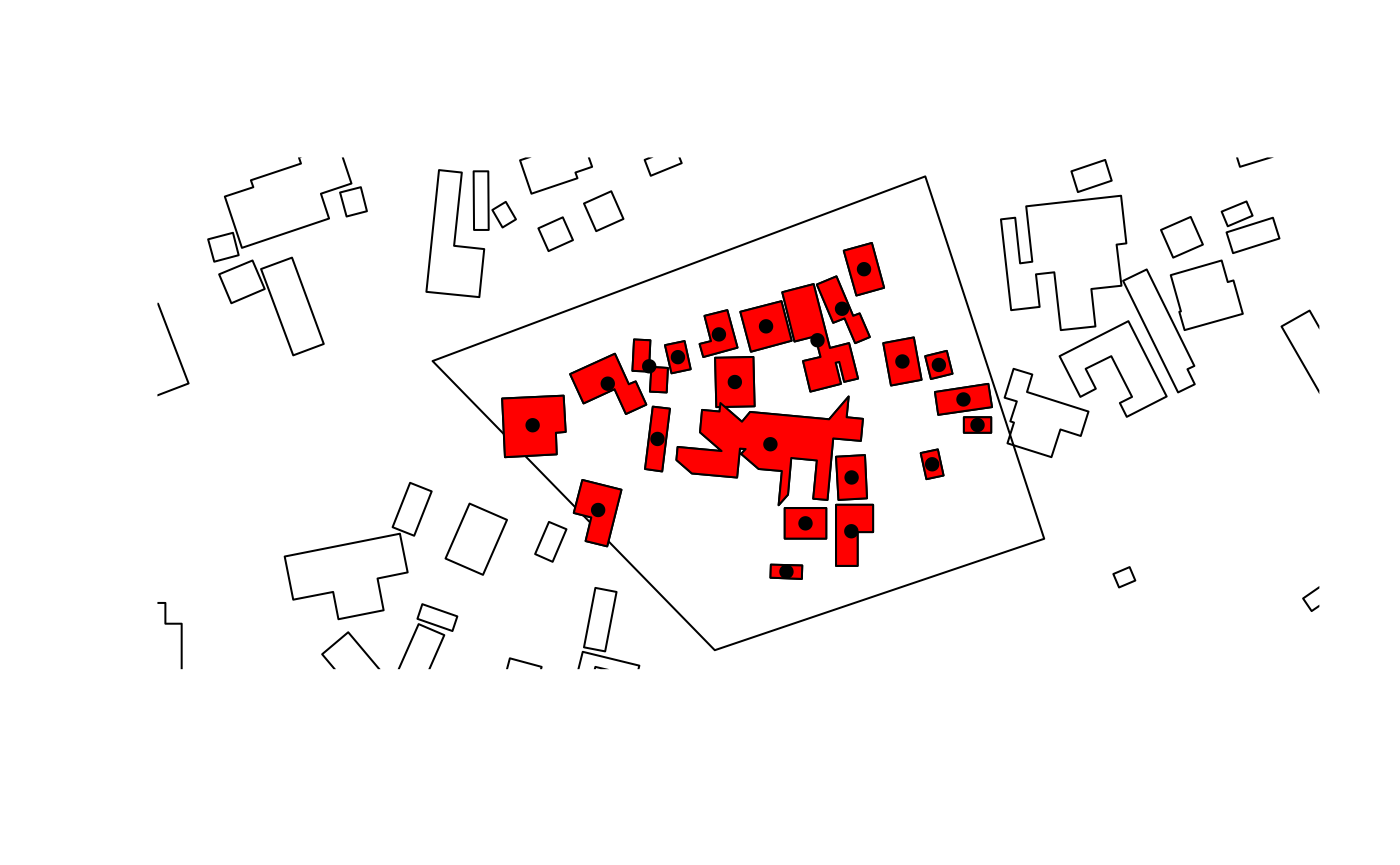
Alternatively, an intersection can be used to assign footprints to any zones which are intersected. The whole footprint is associated, even if the shape is not “contained” by the zone.
# Note the selected structures extend beyond the cluster boundary
zInt <- zonalIndex(buildings, clusters, zoneField = "Id", method = "intersect")

plot(sf::st_geometry(clusters)[[6]])
plot(sf::st_geometry(buildings), add = T)
plot(sf::st_geometry(zInt[zInt$Id == 6, ]), col = "red", add = T)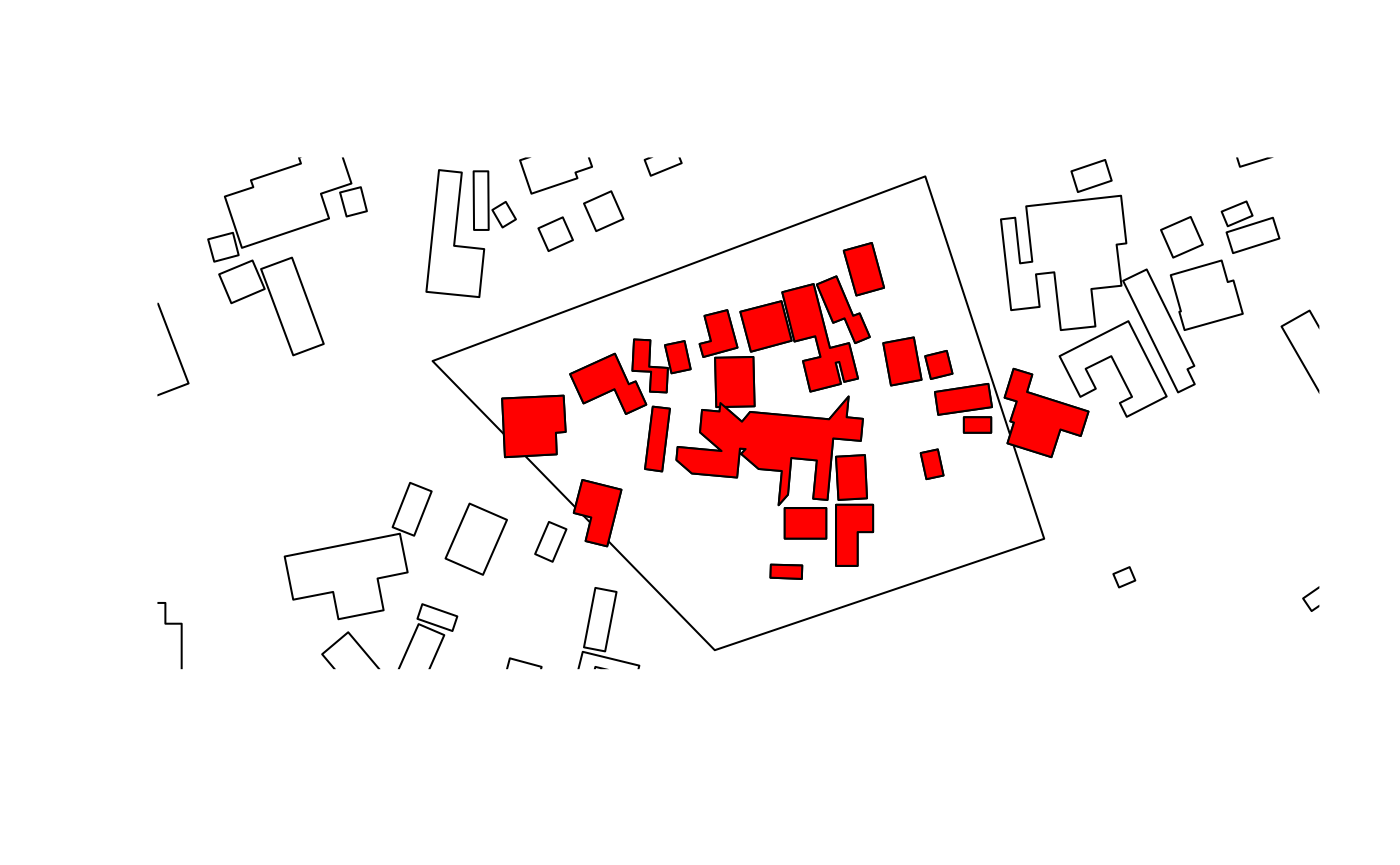
Finally, the intersection can return a clipped set of buildings.
zClip <- zonalIndex(buildings, clusters, zoneField = "Id", method = "clip")

plot(sf::st_geometry(clusters)[[6]])
plot(sf::st_geometry(buildings), add = T)
plot(sf::st_geometry(zClip[zClip$Id == 6, ]), col = "red", add = T)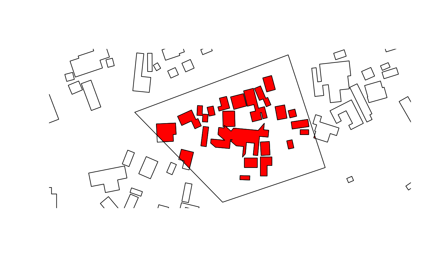
This third option clips the footprints via intersection, potentially leaving small slivers of structures in the zone which will affect the feature statistics.
An additional side effect of the intersection operation is that overlapping zones are allowed, and this can duplicate and associate footprints into both (overlapping) zones.
# create a temporary shape by shifting one cluster
newClusters <- st_sfc(sf::st_geometry(clusters)[[1]], sf::st_cast(sf::st_geometry(clusters)[[1]] +
    c(0.001, 1e-04), "POLYGON"), crs = sf::st_crs(clusters))

newClusters <- st_sf(geometry = newClusters, crs = sf::st_crs(clusters))

newObj <- zonalIndex(buildings, newClusters, method = "clip")

# areas of overlap are in a purple hue
plot(sf::st_geometry(newClusters))
plot(sf::st_geometry(newObj[newObj$zoneID == 1, ]), col = "red", add = T)
plot(sf::st_geometry(newObj[newObj$zoneID == 2, ]), col = sf::sf.colors(n = 1, alpha = 0.5),
    add = T)
plot(sf::st_geometry(buildings), add = T)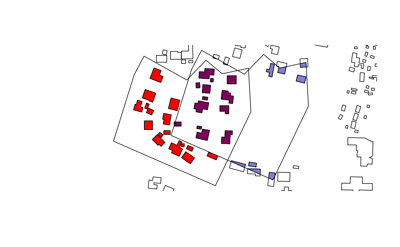
These side effects are allowed because they allow for flexibility to support types of “focal” summaries of statistics and to produce a true gridded measure of footprint metrics.
Calculating multiple metrics
The calculate_footstats() function provides a convenient wrapper to the individual footprint statistics and as well to zonalIndex. The function accepts a variety of input formats (see ?calculate_footstats). Multiple metrics can be calculated for the same sets of buildings and zones.
# Creates a zonal index and calculates multiple metrics
# Use the intersection method define zones
results <- calculate_footstats(buildings,
                               zone=adminzones,
                               what="area",
                               how=list("mean","cv"),
                               controlZone=list(method="intersect"),
                               verbose=F
                              )
  results
#>     zoneID        area_mean   area_cv
#>  1:      1  404.40622 [m^2] 1.2479809
#>  2:      2  212.00113 [m^2] 1.1069491
#>  3:      3  527.43250 [m^2] 1.9194754
#>  4:      4  557.58574 [m^2] 3.8206699
#>  5:      5  571.26921 [m^2] 1.7000587
#>  6:      6 1026.54193 [m^2] 2.0652378
#>  7:      7 2036.80923 [m^2] 1.4077033
#>  8:      8  912.32644 [m^2] 1.4225521
#>  9:      9  182.49803 [m^2] 1.6104922
#> 10:     10  253.12878 [m^2] 1.5272719
#> 11:     11  221.10092 [m^2] 1.4300230
#> 12:     12   88.23133 [m^2] 1.2659927
#> 13:     13  664.58989 [m^2] 1.7191007
#> 14:     14   82.22200 [m^2] 0.3447115
#> 15:     15   81.14808 [m^2] 1.0115881
#> 16:     16   69.06033 [m^2] 0.5102143
#> 17:     17  139.80020 [m^2] 0.8678702
#> 18:     18   87.62864 [m^2] 1.5248900
#> 19:     19  238.14083 [m^2] 0.6189696
#> 20:     20  200.28897 [m^2] 0.9103598
#> 21:     21  245.19516 [m^2] 2.4147823
#> 22:     22  193.25951 [m^2] 0.3464272
#> 23:     23  779.48455 [m^2] 2.1447695
#> 24:     24  220.25691 [m^2] 0.7972001
#> 25:     25  508.49467 [m^2] 1.3228666
#> 26:     26 1143.07662 [m^2] 1.6994280
#> 27:     27  229.03249 [m^2] 2.2623265
#> 28:     29  239.83238 [m^2] 2.7887959
#> 29:     30  204.59597 [m^2] 0.8303153
#> 30:     31  142.77472 [m^2]        NA
#> 31:     32  273.99468 [m^2] 1.0894764
#> 32:     33  420.54389 [m^2] 0.9787568
#> 33:     34  177.61130 [m^2] 1.3707628
#>     zoneID        area_mean   area_cv
Multiple metrics can be applied to specific groups of characteristics by providing nested lists of metrics and summary functions. The argument what will accept a string or a list of strings for specific metric names. Users may also supply "all" or "nodist" to calculate all available metrics or all bar the nearest neighbour distance-related ones, respectively. Excluding the distance-related metrics can speed up the calculations due to the long-running. Other performance improvements can be to set controlDistance=list("method"="centroid"), which uses centroid-to-centroid nearest neighbour distances rather than polygon edge-to-edge. See also, ?fs_nndist.
# Use nested lists to group characteristics and summary functions
results <- calculate_footstats(buildings,
                               zone=adminzones,
                               what=list(list("area","perimeter"),
                                         list("settled")),
                               how=list(list("sum","cv"),
                                        list("count")),
                               controlZone=list(method="centroid"),
                               verbose=F
                              )
  results
#>     zoneID          area_sum   perimeter_sum   area_cv perimeter_cv
#>  1:      1   8492.5307 [m^2]  1781.62245 [m] 1.2479809    0.6561304
#>  2:      2  29892.1595 [m^2]  8596.30974 [m] 1.1069491    0.7313348
#>  3:      3  25844.1923 [m^2]  4414.86934 [m] 1.9194754    0.9811076
#>  4:      4  64122.3606 [m^2]  9640.94681 [m] 3.8206699    1.0600954
#>  5:      5  26849.6529 [m^2]  4329.10334 [m] 1.7000587    0.9581201
#>  6:      6  35928.9675 [m^2]  3835.74843 [m] 2.0652378    0.9616081
#>  7:      7  28515.3292 [m^2]  2565.09927 [m] 1.4077033    0.9286094
#>  8:      8  44703.9953 [m^2]  6348.37632 [m] 1.4225521    0.8489816
#>  9:      9  48361.9770 [m^2] 15739.78807 [m] 1.6104922    0.9246860
#> 10:     10   7593.8634 [m^2]  2087.88260 [m] 1.5272719    1.0900293
#> 11:     11  24321.1016 [m^2]  7672.66021 [m] 1.4300230    0.8815988
#> 12:     12   3123.7687 [m^2]  1403.25960 [m] 1.3014214    0.7257624
#> 13:     13   2658.3596 [m^2]   423.87801 [m] 1.7191007    1.3165558
#> 14:     14   6742.2042 [m^2]  3088.40482 [m] 0.3447115    0.2059276
#> 15:     15  19313.2428 [m^2]  8676.96497 [m] 1.0115881    0.5073846
#> 16:     16   9944.6881 [m^2]  4968.39946 [m] 0.5102143    0.3095971
#> 17:     17  14818.8207 [m^2]  5213.18182 [m] 0.8678702    0.5541695
#> 18:     18  37061.1108 [m^2] 15742.13708 [m] 1.5308487    0.7093738
#> 19:     19  96923.3173 [m^2] 26354.10548 [m] 0.6189696    0.4151437
#> 20:     20  80716.4561 [m^2] 23566.14546 [m] 0.9103598    0.5257108
#> 21:     21  18144.4417 [m^2]  4403.44976 [m] 2.4147823    0.7810948
#> 22:     22  10242.7539 [m^2]  3061.47987 [m] 0.3464272    0.2238327
#> 23:     23 133268.8176 [m^2] 17464.78357 [m] 2.1625263    1.1205392
#> 24:     24  62112.4473 [m^2] 17707.47705 [m] 0.7972001    0.5317242
#> 25:     25  11695.3775 [m^2]  2163.70761 [m] 1.3228666    0.8940386
#> 26:     26 150883.2148 [m^2] 17604.40321 [m] 1.6814458    1.0767096
#> 27:     27  33968.6861 [m^2] 10017.95165 [m] 0.7963207    0.4462858
#> 28:     29  37174.0182 [m^2]  9185.83050 [m] 2.7887959    1.0713172
#> 29:     30  15344.6975 [m^2]  4621.61764 [m] 0.8303153    0.5426390
#> 30:     31    142.7747 [m^2]    48.13661 [m]        NA           NA
#> 31:     32  35893.3028 [m^2]  9127.30909 [m] 1.0894764    0.6469339
#> 32:     33   7149.2461 [m^2]  1557.24261 [m] 0.9787568    0.6104610
#> 33:     34 147594.9907 [m^2] 47733.83601 [m] 1.3707628    0.7474269
#>     zoneID          area_sum   perimeter_sum   area_cv perimeter_cv
#>     settled_count
#>  1:            21
#>  2:           141
#>  3:            49
#>  4:           115
#>  5:            47
#>  6:            35
#>  7:            14
#>  8:            49
#>  9:           265
#> 10:            30
#> 11:           110
#> 12:            36
#> 13:             4
#> 14:            82
#> 15:           238
#> 16:           144
#> 17:           106
#> 18:           424
#> 19:           407
#> 20:           403
#> 21:            74
#> 22:            53
#> 23:           172
#> 24:           282
#> 25:            23
#> 26:           129
#> 27:           177
#> 28:           155
#> 29:            75
#> 30:             1
#> 31:           131
#> 32:            17
#> 33:           831
#>     settled_count
Filtering buildings
In some settings it may be preferable to exclude very small and/or very large building footprint polygons. The lower and upper bounds for filtering can be specified with minArea and maxArea in the filter argument. The values for these filters are in the same units specified by controlUnits or the default value for area calculations. Note that an “area” footprint statistic does not need to be requested as this characteristic is automatically calculated to enable filtering.
# Filtering: # footprints must be larger than 50 m^2 and smaller than 1000 m^2
calculate_footstats(buildings,
                    what="perimeter",
                    how=list("mean", "sum"),
                    controlUnits=list(areaUnit="m^2"),
                    filter=list(minArea=50, maxArea=1000),
                    verbose=FALSE)
#>    zoneID perimeter_mean perimeter_sum
#> 1:      1   63.06881 [m]  228561.4 [m]
Next steps
The calculate_footstats function provides the core functionality for calculating and summarising the characteristics of building footprints. It also wraps the functionality of assigning footprints to zones based on different spatial joining techniques. To go further with foot the concept of footprint morphology calculations can be extended to created gridded data. See vignette("bigfoot", package="foot"). Additionally, users can specify their own custom summary functions to be used with calculate_footstats. This and other advanced options are covered in vignette("cobbler", package="foot").
sessionInfo()
#> R version 4.1.1 (2021-08-10)
#> Platform: x86_64-pc-linux-gnu (64-bit)
#> Running under: Ubuntu 20.04.3 LTS
#>
#> Matrix products: default
#> BLAS:   /usr/lib/x86_64-linux-gnu/blas/libblas.so.3.9.0
#> LAPACK: /usr/lib/x86_64-linux-gnu/lapack/liblapack.so.3.9.0
#>
#> locale:
#>  [1] LC_CTYPE=en_GB.UTF-8       LC_NUMERIC=C
#>  [3] LC_TIME=en_GB.UTF-8        LC_COLLATE=en_GB.UTF-8
#>  [5] LC_MONETARY=en_GB.UTF-8    LC_MESSAGES=en_GB.UTF-8
#>  [7] LC_PAPER=en_GB.UTF-8       LC_NAME=C
#>  [9] LC_ADDRESS=C               LC_TELEPHONE=C
#> [11] LC_MEASUREMENT=en_GB.UTF-8 LC_IDENTIFICATION=C
#>
#> attached base packages:
#> [1] stats     graphics  grDevices utils     datasets  methods   base
#>
#> other attached packages:
#> [1] sf_1.0-0 foot_0.8
#>
#> loaded via a namespace (and not attached):
#>  [1] Rcpp_1.0.7         lattice_0.20-45    class_7.3-19       rprojroot_2.0.2
#>  [5] digest_0.6.28      foreach_1.5.1      utf8_1.2.2         R6_2.5.1
#>  [9] evaluate_0.14      e1071_1.7-7        highr_0.9          pillar_1.6.4
#> [13] rlang_0.4.12       geosphere_1.5-10   data.table_1.14.2  jquerylib_0.1.3
#> [17] rmarkdown_2.11     pkgdown_1.6.1      textshaping_0.3.5  desc_1.4.0
#> [21] geos_0.1.1         stringr_1.4.0      proxy_0.4-26       compiler_4.1.1
#> [25] xfun_0.27          pkgconfig_2.0.3    systemfonts_1.0.3  htmltools_0.5.2
#> [29] tidyselect_1.1.0   tibble_3.1.5       codetools_0.2-18   fansi_0.5.0
#> [33] crayon_1.4.2       dplyr_1.0.5        wk_0.4.1           grid_4.1.1
#> [37] jsonlite_1.7.2     lwgeom_0.2-6       lifecycle_1.0.1    DBI_1.1.1
#> [41] magrittr_2.0.1     formatR_1.11       units_0.7-2        KernSmooth_2.23-20
#> [45] stringi_1.7.5      cachem_1.0.6       libgeos_3.9.1-1    fs_1.5.0
#> [49] sp_1.4-5           doParallel_1.0.16  bslib_0.2.4        ellipsis_0.3.2
#> [53] filelock_1.0.2     ragg_1.1.3         generics_0.1.0     vctrs_0.3.8
#> [57] s2_1.0.6           iterators_1.0.13   tools_4.1.1        glue_1.4.2
#> [61] purrr_0.3.4        abind_1.4-5        parallel_4.1.1     fastmap_1.1.0
#> [65] yaml_2.2.1         stars_0.5-3        classInt_0.4-3     memoise_2.0.0
#> [69] knitr_1.36         sass_0.3.1