The foot package was developed by WorldPop at the University of Southampton (www.worldpop.org) to support geometric calculations and zonal summaries of measures from building footprint polygons. The vignette("footsteps", package="foot") provides an introduction to package and the functionality of calculating and summarising morphology measures. This vignette builds on those methods and demonstrates a more advanced workflow to produce gridded summaries of buildings measures. In particular, the focus is on using foot::calculate_bigfoot() in order how to handle very large (i.e.  national-scale) datasets of building footprints.

An example of this type of processing and how it can be used in settlement classification is available in this paper (open access): https://doi.org/10.1371/journal.pone.0247535.

Calculations with foot

The central function for producing gridded layers is calculate_bigfoot. It is designed to support processing large sets of building polygons into gridded (GeoTiff) summary layers. The procedure is intended to be more memory-efficient by splitting the processing area into “tiles” which can then be handled individually or in parallel. This function works as a wrapper to calculate_footstats as well as several helper functions within the foot package for managing the input/output and creating and indexing spatial zones. Because it extends calculate_footstats, this function takes the same what= and how= arguments to define the summary operations. Likewise the available metrics are available from list_fs().

By default the function performs calculations in parallel (which can be changed with the argument parallel=FALSE). Users can adjust the number of computing cores used with the argument nCores=) To monitor the supplied values and processing steps, set verbose=TRUE.

Main inputs

Users need to supply calculate_bigfoot() with:

  • A path to a file of building footprints in a spatial vector data format (e.g. .gpkg, .shp)
  • A filepath to a template gridded dataset specifying the extent and resolution for the outputs (e.g. .tif)

For example:

While R objects can be supplied for the function parameters (as will be shown in this example), it is recommended to supply character strings of paths to the files. calculate_bigfoot will only read the subset of data needed for a particular processing step. This is intended to allow users to process much larger datasets than can be held in memory.

Basic calculations

With the key inputs for the file paths set, the processing can be executed with a single function.

# basic function call with default parameters
calculate_bigfoot(X=buildings,
                  template=mgrid,
                  what="settled", how="binary",
                  parallel=FALSE, verbose=TRUE)
#> Reading template grid 
#> trying to read file: C:\Users\Admin\Documents\GitHub\foot\wd\in\kampala_grid.tif
#> Selecting metrics 
#> Setting control values 
#> Creating output grids 
#> Creating list of processing tiles 
#> 
#> Tile: 1 of 1
#> Reading footprints 
#> Reading template grid 
#> Selecting metrics 
#> Setting control values. 
#> Creating zonal index 
#> 
#> Calculating  1  metrics ... 
#>    settled binary  
#> Finished calculating metrics. 
#> Writing output tiles 
#> Finished writing grids
#> 
#> Finished processing all tiles: 2021-11-10 18:01:55

The documentation and default parameters are available from ?foot::calculate_bigfoot.

The arguments what and how are the same as for calculate_footstats. They provide a character or list list of character names or characteristics (i.e. columns within the building footprint attributes) and summary functions, respectively. The available metrics can be retrieved with list_fs().

Specifying outputs

By default the outputs of bigfoot are saved as GeoTiffs in the user’s working directory (getwd()). Each grid is named by the combination of characteristics and summary function. The example below shows how to retrieve an output of calculate_bigfoot.

# retrieve the gridded outputs
outGrid <- raster::raster(file.path(getwd(), "settled_binary.tif"))

raster::plot(outGrid)
Binary settled raster at 100m resolution

Binary settled raster at 100m resolution

Users can specify an output path to another folder location (outputPath=). Additionally a “tag” can be specified as a parameter to the function (outputTag=). The tag is appended to the beginning of each file name with an underscore. This can be useful for identifying different outputs. These options are demonstrated in the code block below.

# basic function call specifying output parameters
calculate_bigfoot(X=buildings,
                  template=mgrid,
                  what="settled", how="binary",
                  outputPath=tempdir(),
                  outputTag="TAG",
                  parallel=FALSE, verbose=TRUE)
#> Reading template grid 
#> trying to read file: C:\Users\Admin\Documents\GitHub\foot\wd\in\kampala_grid.tif
#> Selecting metrics 
#> Setting control values 
#> Creating output grids 
#> Creating list of processing tiles 
#> 
#> Tile: 1 of 1
#> Reading footprints 
#> Reading template grid 
#> Selecting metrics 
#> Setting control values. 
#> Creating zonal index 
#> 
#> Calculating  1  metrics ... 
#>    settled binary  
#> Finished calculating metrics. 
#> Writing output tiles 
#> Finished writing grids
#> 
#> Finished processing all tiles: 2021-11-10 18:01:58

Multiple metrics

As with calculate_footstats multiple metrics and summary statistics can be supplied to bigfoot as a list or nested lists grouping characteristics and functions.

# re-running the basic call with multiple metrics
calculate_bigfoot(X=buildings,
                  template=mgrid, 
                  what=list(list("settled"), list("area")),
                  how=list(list("binary"), list("cv")),
                  outputPath=tempdir(),  
                  outputTag="TAG", parallel=FALSE)  
#> Reading template grid 
#> trying to read file: C:\Users\Admin\Documents\GitHub\foot\wd\in\kampala_grid.tif
#> Selecting metrics 
#> Setting control values 
#> Creating output grids 
#> Creating list of processing tiles 
#> 
#> Tile: 1 of 1
#> Reading footprints 
#> Reading template grid 
#> Selecting metrics 
#> Setting control values. 
#> Pre-calculating areas 
#> Creating zonal index 
#> 
#> Calculating  2  metrics ... 
#>    settled binary  
#>    area cv  
#> Finished calculating metrics. 
#> Writing output tiles 
#> Finished writing grids
#> 
#> Finished processing all tiles: 2021-11-10 18:02:01
# retrieve the gridded outputs Note: must add the 'tag' to the filename
outGrid <- raster::raster(file.path(tempdir(), "TAG_area_cv.tif"))

raster::plot(outGrid)
plot(sf::st_geometry(buildings), fill = NA, add = T)
Coeff. of variation in building area at 100m resolution

Coeff. of variation in building area at 100m resolution

Focal window statistics

In the examples above, the footprint statistics are summarised for buildings whose centroid intersect the pixels of the template grid. Internally this is handled by zonalIndex(). The method for assigning footprints to spatial zones can be adjusted using controlZone options.

It is also possible to extend those zones beyond the individual pixels and to calculate and summarise building footprints from within a local, circular window centred on each pixel. The output is still associated with each template grid cell. This process is similar to a moving window or filter analysis. The focal radius distance is specified in meters.

A hypothetical example of using a 300 m focal radius around a pixel centroid to construct a local zone and using building centroids is shown below.
Example of 300 m focal radius. Selected footprints are highlighted in red

Example of 300 m focal radius. Selected footprints are highlighted in red

Below is an example of applying a 300 m focal radius in action for a gridded output layer.

# moving focal window calculations
calculate_bigfoot(X=buildings,
                  template=mgrid,
                  what=list(list("area"), list("perimeter")),
                  how=list(list("mean"), list("sum")),
                  focalRadius=300,  # buffer radius in meters
                  outputPath=tempdir(), 
                  outputTag="TAG", parallel=FALSE)
#> Reading template grid 
#> trying to read file: C:\Users\Admin\Documents\GitHub\foot\wd\in\kampala_grid.tif
#> Selecting metrics 
#> Setting control values 
#> Creating output grids 
#> Creating list of processing tiles 
#> 
#> Tile: 1 of 1
#> Reading footprints 
#> Reading template grid 
#> Buffering processing sites 
#> Selecting metrics 
#> Setting control values. 
#> Pre-calculating areas 
#> Pre-calculating perimeters 
#> Creating zonal index 
#> 
#> Calculating  2  metrics ... 
#>    area mean  
#>    perimeter sum  
#> Finished calculating metrics. 
#> Writing output tiles 
#> Finished writing grids
#> 
#> Finished processing all tiles: 2021-11-10 18:02:08

Creating the focal window is handled by calculate_bigfoot. The focal window is also taken into consideration by the function when creating processing tiles - the footprints are extract from outside the tile, in neighbouring areas, to prevent edge effects

Note that when a focal radius is specified, this value is always appended to the end of the file names so that the outputs can be identified.

# Note that the filename includes both a tag and a focal radius value
outGrid <- raster::raster(file.path(tempdir(), "TAG_perimeter_sum_300.tif"))

raster::plot(outGrid)
Total building perimeter in a 300m radius window. Output at a 100m resolution

Total building perimeter in a 300m radius window. Output at a 100m resolution

Options and finer control

The calculate_bigfoot function is set up with default values that should work under most conditions; however, there is additional flexibility for users to specify alternative parameters.

Specifying geometry units

To override the default units used in the geometry calculations, a named list of unit strings can be supplied to the controlUnits argument. This list can contain named items for areaUnit, perimUnit, and distUnit. The default values are meters (“m”) and square meters (“m^2”) The value of each item should be coercible with units::as_units.

# change the default units used to calculate area and distance
calculate_bigfoot(X=buildings,
                  template=mgrid, 
                  what=list(list("area"), list("perimeter")),
                  how=list(list("mean"), list("sum")),
                  controlZone=list("method"="intersect"), # join by intersection
                  controlUnits=list(areaUnit="m^2",  # change default units
                                    perimUnit="km"),
                  outputPath=tempdir(),  
                  outputTag="TAG",
                  parallel=FALSE,
                  verbose=TRUE)  
#> Reading template grid 
#> trying to read file: C:\Users\Admin\Documents\GitHub\foot\wd\in\kampala_grid.tif
#> Selecting metrics 
#> Setting control values 
#> Creating output grids 
#> Creating list of processing tiles 
#> 
#> Tile: 1 of 1
#> Reading footprints 
#> Reading template grid 
#> Selecting metrics 
#> Setting control values. 
#> Pre-calculating areas 
#> Pre-calculating perimeters 
#> Creating zonal index 
#> 
#> Calculating  2  metrics ... 
#>    area mean  
#>    perimeter sum  
#> Finished calculating metrics. 
#> Writing output tiles 
#> Finished writing grids
#> 
#> Finished processing all tiles: 2021-11-10 18:02:12

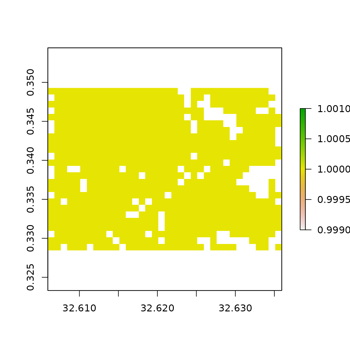
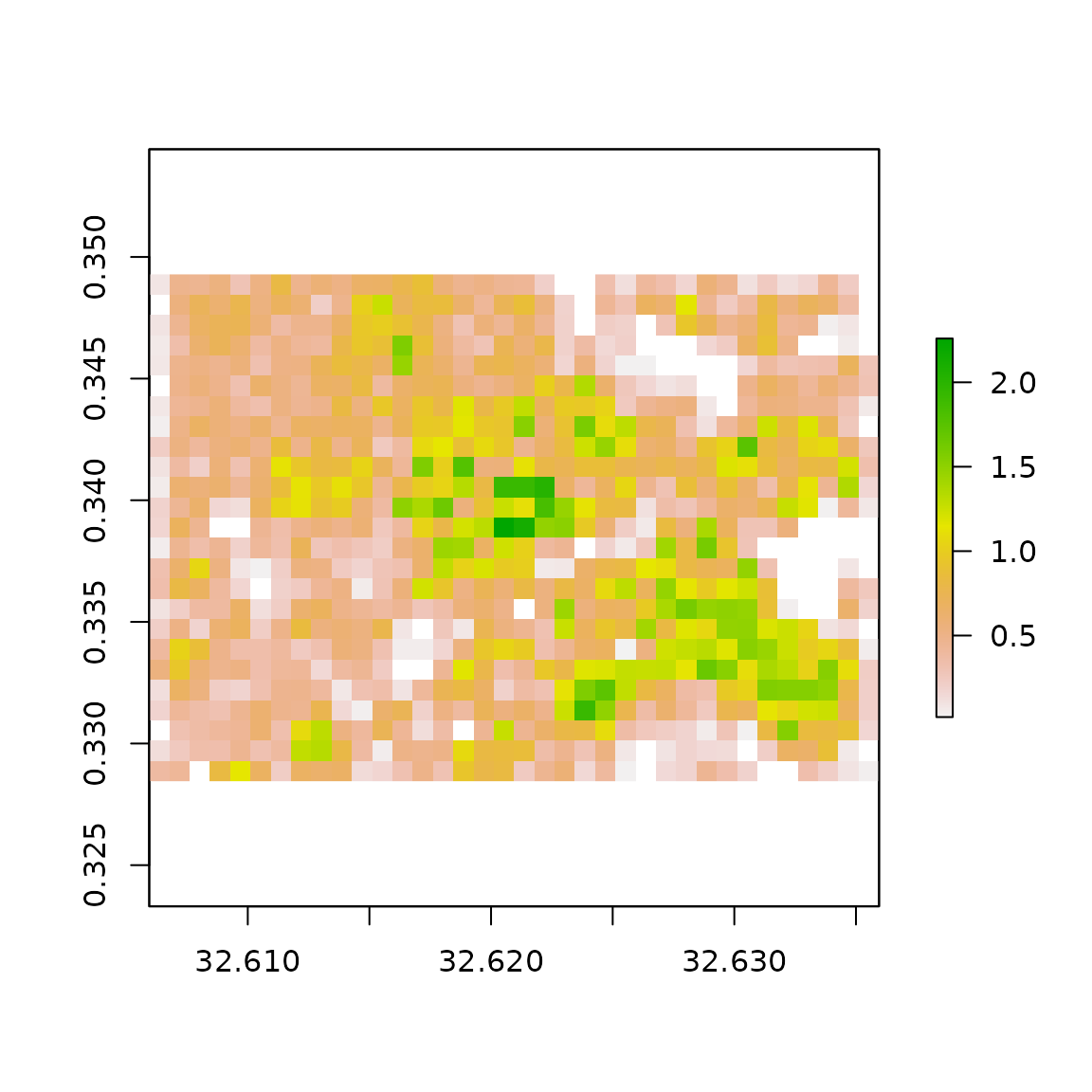
# plot the total perimeter, measured in kilometres
outGrid <- raster::raster(file.path(tempdir(), "TAG_perimeter_sum.tif"))
raster::plot(outGrid)
Total building perimeter in KM

Total building perimeter in KM

Filtering buildings

In some settings it may be preferable to exclude very small and/or very large building footprint polygons. The lower and upper bounds for filtering can be specified with minArea and maxArea in the filter argument. The values for these filters are in the same units specified by controlUnits or the default value for area calculations. Note that an “area” footprint statistic does not need to be requested as this characteristic is automatically calculated to enable filtering.

# Filtering: # footprints must be larger than 50 m^2 and smaller than 1000 m^2
calculate_bigfoot(X=buildings,
                  template=mgrid, 
                  what=list(list("shape"), list("settled"), list("perimeter")),
                  how=list(list("mean"), list("count"), list("sum")),
                  controlUnits=list(areaUnit="m^2"),
                  filter=list(minArea=50, maxArea=1000),
                  outputPath=tempdir(),  
                  parallel=FALSE,
                  verbose=TRUE)  
#> Reading template grid 
#> trying to read file: C:\Users\Admin\Documents\GitHub\foot\wd\in\kampala_grid.tif
#> Selecting metrics 
#> Setting control values 
#> Creating output grids 
#> Creating list of processing tiles 
#> 
#> Tile: 1 of 1
#> Reading footprints 
#> Reading template grid 
#> Selecting metrics 
#> Setting control values. 
#> Pre-calculating areas 
#> Pre-calculating perimeters 
#> Pre-calculating shape 
#> Creating zonal index 
#>  Filtering features larger than 50 
#>  Filtering features smaller than 1000 
#> 
#> Calculating  3  metrics ... 
#>    shape mean  
#>    settled count  
#>    perimeter sum  
#> Finished calculating metrics. 
#> Writing output tiles 
#> Finished writing grids
#> 
#> Finished processing all tiles: 2021-11-10 18:02:20

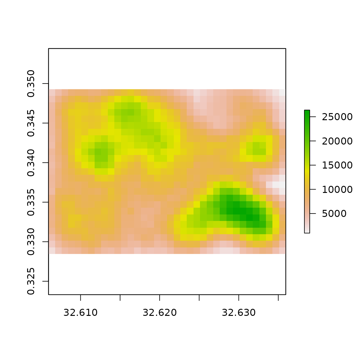
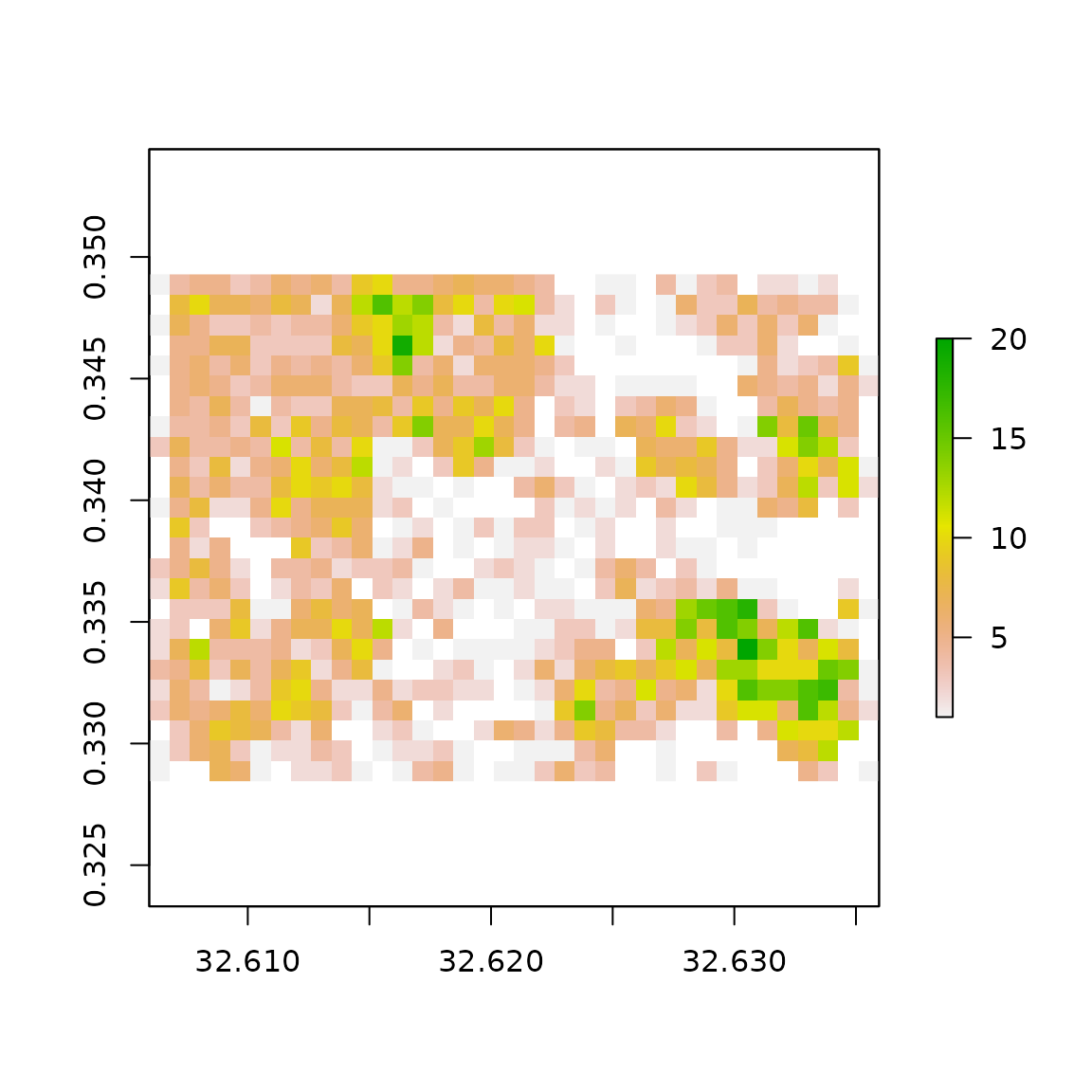
In the map of the results below, each pixel is the count of footprints present. Note the smaller number of structures and sparseness of structures in pixels around the centre portions of the image. This corresponds with the a business district and industrial areas with fewer, but larger structures.

outGrid <- raster::raster(file.path(tempdir(), "settled_count.tif"))

raster::plot(outGrid)
Count of buildings with area >50 m^2 and <1000 m^2

Count of buildings with area >50 m^2 and <1000 m^2

Tile size

The size of the processing tiles, specified in pixel dimensions (rows, columns) can be an important factor in the efficiency of the calculations. Smaller tile regions result in fewer building footprints being read/processed at one time, but there is an overhead computational cost of reading/writing files. The default value is 500 pixels. For the small demonstration shown here that results in one tile for the whole region. To show multiple tile processing, a small size is supplied and the processing is done in parallel with verbose output.

calculate_bigfoot(X=buildings,
                  template=mgrid,
                  what="compact",
                  how="mean",
                  tileSize=c(20, 20),  # rows x columns in pixels
                  parallel=FALSE,
                  verbose=TRUE)
#> Reading template grid 
#> trying to read file: C:\Users\Admin\Documents\GitHub\foot\wd\in\kampala_grid.tif
#> Selecting metrics 
#> Setting control values 
#> Creating output grids 
#> Creating list of processing tiles 
#> 
#> Tile: 1 of 4
#> Reading footprints 
#> Reading template grid 
#> Selecting metrics 
#> Setting control values. 
#> Pre-calculating compactness 
#> Creating zonal index 
#> 
#> Calculating  1  metrics ... 
#>    compact mean  
#> Finished calculating metrics. 
#> Writing output tiles 
#> Finished writing grids
#> 
#> Tile: 2 of 4
#> Reading footprints 
#> Reading template grid 
#> Selecting metrics 
#> Setting control values. 
#> Pre-calculating compactness 
#> Creating zonal index 
#> 
#> Calculating  1  metrics ... 
#>    compact mean  
#> Finished calculating metrics. 
#> Writing output tiles 
#> Finished writing grids
#> 
#> Tile: 3 of 4
#> Reading footprints 
#> Reading template grid 
#> Selecting metrics 
#> Setting control values. 
#> Pre-calculating compactness 
#> Creating zonal index 
#> 
#> Calculating  1  metrics ... 
#>    compact mean  
#> Finished calculating metrics. 
#> Writing output tiles 
#> Finished writing grids
#> 
#> Tile: 4 of 4
#> Reading footprints 
#> Reading template grid 
#> Selecting metrics 
#> Setting control values. 
#> Pre-calculating compactness 
#> Creating zonal index 
#> 
#> Calculating  1  metrics ... 
#>    compact mean  
#> Finished calculating metrics. 
#> Writing output tiles 
#> Finished writing grids
#> 
#> Finished processing all tiles: 2021-11-10 18:02:27

Restarting

When running parallel processes on clusters, it is not currently possible to show a progress bar. This issue will hopefully be addressed in the future. However, when verbose=TRUE, bigfoot will write a log file to the output directory with the gridded data. This file is a list of tile ID numbers that have been processed. Tiles (created with gridTiles) are numbered sequentially from top-left to bottom-right of the template grid. On long-running jobs, the log of completed tiles can be used to monitor progress. Note that each processor will write its results as they are finished, so tiles may not be completed in order.

If a processing job crashes, the log file can also be used to restart the job. Setting the argument restart to a number will restart processing from that tile. Alternatively a sequence of numbers, given as a vector, can be used to re-run only certain tiles. The output grids will not be overwritten when restarting.

Next steps

This vignette has provided an overview of how to create gridded outputs layers summarising building footprint morphology measures. This workflow uses calculate_bigfoot and is designed to work for large sets of data through tiled read/writing and processing these tiles in parallel. The bigfoot functionality extends and makes use of footstats. Both of these functions can take use-supplied and custom summary functions. This advanced usage is demonstrated in vignette("cobbler", package="foot").


sessionInfo()
#> R version 4.1.1 (2021-08-10)
#> Platform: x86_64-pc-linux-gnu (64-bit)
#> Running under: Ubuntu 20.04.3 LTS
#> 
#> Matrix products: default
#> BLAS:   /usr/lib/x86_64-linux-gnu/blas/libblas.so.3.9.0
#> LAPACK: /usr/lib/x86_64-linux-gnu/lapack/liblapack.so.3.9.0
#> 
#> locale:
#>  [1] LC_CTYPE=en_GB.UTF-8       LC_NUMERIC=C              
#>  [3] LC_TIME=en_GB.UTF-8        LC_COLLATE=en_GB.UTF-8    
#>  [5] LC_MONETARY=en_GB.UTF-8    LC_MESSAGES=en_GB.UTF-8   
#>  [7] LC_PAPER=en_GB.UTF-8       LC_NAME=C                 
#>  [9] LC_ADDRESS=C               LC_TELEPHONE=C            
#> [11] LC_MEASUREMENT=en_GB.UTF-8 LC_IDENTIFICATION=C       
#> 
#> attached base packages:
#> [1] stats     graphics  grDevices utils     datasets  methods   base     
#> 
#> other attached packages:
#> [1] sf_1.0-0     raster_3.4-5 sp_1.4-5     foot_0.8    
#> 
#> loaded via a namespace (and not attached):
#>  [1] Rcpp_1.0.7         lattice_0.20-45    class_7.3-19       rprojroot_2.0.2   
#>  [5] digest_0.6.28      foreach_1.5.1      utf8_1.2.2         R6_2.5.1          
#>  [9] evaluate_0.14      e1071_1.7-7        highr_0.9          pillar_1.6.4      
#> [13] rlang_0.4.12       data.table_1.14.2  jquerylib_0.1.3    rmarkdown_2.11    
#> [17] pkgdown_1.6.1      textshaping_0.3.5  desc_1.4.0         rgdal_1.5-23      
#> [21] stringr_1.4.0      proxy_0.4-26       compiler_4.1.1     xfun_0.27         
#> [25] pkgconfig_2.0.3    systemfonts_1.0.3  htmltools_0.5.2    tidyselect_1.1.0  
#> [29] tibble_3.1.5       codetools_0.2-18   fansi_0.5.0        crayon_1.4.2      
#> [33] dplyr_1.0.5        wk_0.4.1           grid_4.1.1         jsonlite_1.7.2    
#> [37] lwgeom_0.2-6       lifecycle_1.0.1    DBI_1.1.1          magrittr_2.0.1    
#> [41] formatR_1.11       units_0.7-2        KernSmooth_2.23-20 stringi_1.7.5     
#> [45] cachem_1.0.6       fs_1.5.0           doParallel_1.0.16  bslib_0.2.4       
#> [49] ellipsis_0.3.2     filelock_1.0.2     ragg_1.1.3         generics_0.1.0    
#> [53] vctrs_0.3.8        s2_1.0.6           iterators_1.0.13   tools_4.1.1       
#> [57] glue_1.4.2         purrr_0.3.4        abind_1.4-5        parallel_4.1.1    
#> [61] fastmap_1.1.0      yaml_2.2.1         stars_0.5-3        classInt_0.4-3    
#> [65] memoise_2.0.0      knitr_1.36         sass_0.3.1