jollofR

1. Background

jollofR version 0.3.0 is an R package that enables rapid disaggregation of small area population estimates into demographic groups such as age and sex classes as well as other socio-demographic and socio-economic categories (e.g., marital status, wealth indices, educational level, etc). It facilitates the filling of important population data gaps especially across settings where census data are either outdated or incomplete. jollofR is based on advanced multi-steps Bayesian hierarchical statistical modelling approach which first estimates the proportions of each demographic group’s composition within the population of interest based on a (often partially observed) sample data, and then uses it to disaggregate the total population estimate for each administrative unit within the population. jollofR also includes functions to easily disaggregate the population proportions and population numbers at high-resolution grid cells (e.g., 100m by 100m) along with the corresponding estimates of uncertaintity thereby facilitating evidence-based decision-making at small area units. It is fully automated and does not require any special skills or deep knowledge in statistics or statistical modelling, and the input population datasets could come from various sources including census, census projections, Microcensus, household surveys and administrative records.

This statistical model-based approach allows us to estimate population proportions and population counts across all the demographic units of interest including at locations with no observations within the sample data. The use of Bayesian inference approach enables easy quantification of uncertainties in the model parameter estimates based on the 95% credible interval of the posterior distribution. Within the jollofR package, the posterior inference is formulated on the integrated nested Laplace approximation (INLA; Rue et al., 2009) techniques in conjunction with the stochastic partial differential equation (SPDE; Lindgren et al., 2011) strategies, thereby enabling significantly high computational speed. This helps to position the jollofR package as a fast and efficient tool for the rapid production of spatially-structured (e.g., age, sex, ethnicity, wealth, education) population counts and population proportions at small area scales often required for evidence-based governance and more effective humanitarian response efforts. The package is specifically designed to support population data producers and users as well as policymakers in providing timely and spatially detailed small area population data for filling population data gaps across many settings where census is unaffordable due to high cost or where a recent census is incomplete due to the presence of ‘hard-to-reach’ or ‘hard-to-count’ areas as a result of widespread conflicts/unrests or other reasons.

Altogether, the jollofR package contains 14 ‘simplified’ functions and a ‘toy’ dataset to illustrate its implementations across different scenarios. These include functions for population prediction and disaggregation at the administrative units level (‘cheesecake’, ‘cheesepop’, ‘spices’ & ‘slices’) and those used for disaggregation at grid-cell level (‘sprinkle’, ‘sprinkle1’, ‘splash’, ‘splash1’, ‘spray’ & ‘spray1’). Other functions (‘boxLine’, ‘plotHist’, ‘plotRast’ & ‘pyramid’) available within the jollofR package are used for data visualization which enable quick visual assessments of the disaggregated estimates. These functions which are embedded within a robust statistical modelling framework automatically create subnational demographically structured population counts and proportions tables as well as the corresponding high-resolution grid cell raster files in a very simple and efficient manner.

Further details on these functions, their arguments, usage and examples are provided in Section 5 of this document, while further details on the underlying statistical methods are provided in Section 9. Finally, while jollofR could be used to disaggregate population counts and population proportions across any mutually exclusive and exhaustive groups, here, our data description and usage examples are based on age-sex disaggregation, for ease of exposition. Note that, ‘mutually exclusive’ means that every individual within the population is only allowed to belong to one of the non-overlapping groups, while ‘exhaustive’ means that every individual within the entire population must belong to one of the groups and no one is left out. The jollofR functions are designed to be fully flexible to allow for a straightforward implementation for other socio-economic and socio-demographic groups so long as the ‘mutually exclusive and exhaustive’ requirements are met.

2. Installation

System Requirements

Before installing jollofR, please ensure that your system meets the following requirements:

R version: >= 4.1.0
INLA (please check that you have INLA already installed)

Platform-Specific Setup

Windows

Install Rtools (matches your R version):

# Check if Rtools is installed and properly configured
pkgbuild::has_build_tools()

If FALSE, download and install Rtools from: CRAN Rtools

macOS

Install Command Line Tools:

xcode-select --install

Alternatively, install gcc via Homebrew:

brew install gcc

Linux (Ubuntu/Debian)

Update your system and install necessary packages:

sudo apt-get update
sudo apt-get install build-essential libxml2-dev

Install from GitHub

Once the setup is complete, follow the instructions below to download jollofR. Note that the package is still under development. So, we will show you how to install the development version and how to install it once it becomes available on CRAN.

First, you may need to install INLA by running the following codes (if you do not have INLA already installed) ```{r eval=FALSE, include=TRUE}

install.packages(“devtools”)

install.packages(“INLA”, repos=c(getOption(“repos”), INLA=”https://inla.r-inla-download.org/R/stable”), dep=TRUE)

After confirming that **INLA** has been successfully installed, please install the development version of **jollofR** package from GitHub using the following codes: 
```{r eval=FALSE, include=TRUE}
# install.packages("devtools")
devtools::install_github("wpgp/jollofR")

Install from CRAN

As soon as jollofR becomes available on CRAN, you can then install it directly from CRAN using the following: ```{r eval=FALSE, include=TRUE}

install.packages(“jollofR”)

## Other dependencies
In addition to **INLA** package, you may also need to confirm that you have the following packages installed successfully after installing **jollofR**
```{r eval=FALSE, include=TRUE}
library(INLA)
library(jollofR)
library(ggplot2) # use install.packages("ggplot2") to install, if not available
library(dplyr)   # use install.packages("dplyr") to install, if not available
library(terra)   # use install.packages("terra") to install, if not available
library(raster)  # use install.packages("raster") to install, if not available

3. Workflow Overview

jollofR is designed to provide a very simple, efficient and statistically robust appraoch for providing disaggregated population counts across various demographic groups at operational admnistrative unit levels thus making it handy for the production of rapid demographically structured small area population counts. The jollofR package allows for population disaggregation with or without geospatial covariates. However, note that these geospatial covariates are those indentified apriori to significantly predict population distributions (functions which allow for wider range of geospatial covariates and automatically selects and retains the best fit covariates within the package are being developed by the authors). In all cases, estimates of uncertainties are also produced, and boxplots, line graphs, maps, and age-sex pyramid graphs (for age-sex disaggregations) are automatically generated. Below is the flowchart (Figure 1) for the key stages involved in the implementation of the jollofR package.

graph TD;
A[Install INLA and jollofR]-->B[Prepare the input data];
B[Prepare the input data]-->C[Specify the output folder];
C[Specify the output folder]-->D[Run the desired functions];
D[Run the desired functions]-->E[Collate results];

Figure 1: Flowchart of jollofR implementation steps.

Initialise

As a first requirement, you will need to do the following: 1) ensure that you have INLA and jollofR packages installed; 2) create your output folder which is where all the model outputs (results) will be saved, and check to confirm that it works; 3) prepare your input data to ensure it conforms with the input data structure requirements (see the simple data format described within the Preparing the input data section). Once all the initial checks are completed (INLA & jollofR installed and working, input data prepared in the correct formats and structure), you are set to start! Please note that while R GUI could be used, RStudio is highly recommended as it makes it easier to monitor the progress of the computations.

Creating output folder

This is where all the automatically produced outputs will be saved on your machine:

output_dir <- "your output directory"

The package will create the folder if it does not already exist.

Preparing the input data

The input data ‘df’ is a .csv file data frame which contains the key variables of the interest. The data is often a completely anonymized aggregated population data with the following fields:

id: a numeric variable used as the indentification number for each administrative unit (mandatory).
x1, …, xn: n geospatial covariates identified for the covariates-based modelling, i.e., for population disaggregation using covariates. In the ‘toydata’ used as an example here, only 3 geospatial covariates x1, x2, x3 were used for the purpose of illustration only. The package allows for as many covariates as possible in the model. However, please note that the use of covariates to disaggregate a model-based total population estimates, couls lead to circularity issues. Examples of these geospatial covariates include night time light intensity, distance to market, etc - mandatory if disaggregating based on covariates or optional if disaggregating without covariates.
total: an integer valued variable which contains the values to be disggregated. It is the total number of individuals per given administrative unit. Check to ensure that total has values across all the administrative unit of interest. You may wish to first predict all missing total values (mandatory).
age_1, ….., age_n: n age groups of interest containing observed population counts per age group per administrtaive unit. Note that age_1, ….., age_n can come from a sample survey, opportunistically generated data or from incomplete census data. jollofR predicts any missing age proportion, and the these are used to disaggregate the total population count. - mandatory
fage_1, ….., fage_n: n age groups of interest containing observed population counts per age group of females per administrtaive unit. Note that fage_1, ….., fage_n can come from a sample survey, opportunistically generated data or from incomplete census data. jollofR predicts any missing age proportion, and the these are used to disaggregate the total population count.- mandatory
mage_1, ….., mage_n: n age groups of interest containing observed population counts per age group of males per administrtaive unit. Note that mage_1, ….., mage_n can come from a sample survey, opportunistically generated data or from incomplete census data. jollofR predicts any missing age proportion, and the these are used to disaggregate the total population count.

4. Toy data

Toydata

Description

Artificially generated toy datasets that come in a cross-sectional format. The ‘admin’ data is a dataframe collated at administrative unit level which contains information on the observed number of individuals per group (e.g., age and sex groups) within each administrative unit. Key variables include the administrative unit identifier (admin_id), the admin total population to be disaggregated (total), the total number of buildings within each admin unit (bld), and the longitude (lon) and latitude (lat). The ‘admin’ data provides artificial information for 900 spatially distinct administrative units in which the individuals in the population are grouped into 12 mutually exclusive and exhaustive age groups. Each of the age groups was further grouped into ‘male’ and ‘female’ groups. The data contains the total population counts (total) for each spatial unit but also contains missing age and sex groups population counts. The model first predicts the population proportions of the missing data and then disaggregates the population totals using the predicted proportions to obtain the predicted population counts for the age and sex groups. Note that the same applies for other demographic groups such as marital status, race, etc.

Usage

data(toydata)

Format

An object of class “list”- a list object containing two dataframes - an administrative-level dataset (admin) containing partially observed age-sex structured data, and a grid-cell level dataset (grid) for population disaggregation at 1km by 1km grid cells.

admin_id: Available in both the ‘admin’ and ‘grid’ datasets. It is a numerical value which serves as the administrative units unique identifier. They should match perfectly for both the ‘admin’ and grid’ datasets
grd_id: Available in the ‘grid’ dataset only. It is a numerical value which serves as the grid cell unique indentifier.
x1, x2, x3: These are the samples of geospatial covariates (only required for the ‘cheesecake’ and the ‘slices’ functions). Note that these are the covariates identified to significantly predict population distribution among the demographic groups. The package allows the user to include any number of covariates in their own datasets.
total: Available in both the ‘admin’ and ‘grid’ datasets. It provides estimates of the total population counts to be disaggregated. It DOES NOT necessarily have to be a rowsum of the age groups totals.
bld: Available in both the ‘admin’ and ‘grid’ datasets. It provides the total number of buildings in each grid cell or administrative unit.
age_1, …, age_12: These correspond to the partially or fully observed number of people for each age group. Note that only 12 age groups are used here for illustration purposes,however, the package can accommodate any number of age or sex or any demographic groups.
fage_1, …, fage_12: These correspond to the partially or fully observed number of females corresponding to each of the age groups. Note that only 12 age groups are used here for illustration purposes,however, the package can accommodate any number of age or sex or any demographic groups.
mage_1, …, mage_12: These correspond to the partially or fully observed number of males corresponding to each of the age groups. Note that only 12 age groups are used here for illustration purposes,however, the package can accommodate any number of age or sex or any demographic groups.
lon: Available in both the ‘admin’ and ‘grid’ datasets. Provides the value of the longitude of the centroids of the grid cells or admin unit polygons.
lat: Available in both the ‘admin’ and ‘grid’ datasets. Provides the value of the latitude of the centroids of the grid cells or admin unit polygons.

Details:

The ‘admin’ data is used to fit statistical models to predict subnational population estimates and proportions across various groups, while the ‘grid’ data is used for the prediction of the disggregatted population structures at high resolution grid cells. Within the jollofR package the grid data used within the toydata provides estimates of population numbers and proportions at 1km-by-1km spatial resolution. However, jollofR allow for structured population predictions at any spatial resolution of interest. The ‘grid’ data contains six key variables - the administrative unit identifier (admin_id) which must be identical to the those in the ‘admin’ data; the grid cell identifier (grd_id); the total number of people per grid cell (total), if available; the total number of buildings per grid cell (bld), if available; and the longitude (lon) and latitude (lat) variables for the grid cell centroids.

Example

data(toydata)
admin_data <- toydata$admin # subset the admin data

str(admin_data)   # view the structure of the administrative data
'data.frame':	900 obs. of  45 variables:
 $ admin_id: int  1 2 3 4 5 6 7 8 9 10 ...
 $ x1      : num  0.503 0.516 0.493 0.477 0.456 ...
 $ x2      : num  0.472 0.446 0.495 0.451 0.382 ...
 $ x3      : num  0.526 0.613 0.473 0.537 0.562 ...
 $ bld     : int  238 271 276 237 228 226 266 232 215 235 ...
 $ total   : int  2491 2040 1870 2240 2385 2511 3820 3598 3161 3125 ...
 $ age_1   : int  164 NA NA 180 NA NA NA NA 221 209 ...
 $ age_2   : int  159 NA NA 175 NA NA NA NA 227 255 ...
 $ age_3   : int  394 NA NA 344 NA NA NA NA 460 408 ...
 $ age_4   : int  395 NA NA 338 NA NA NA NA 435 425 ...
 $ age_5   : int  253 NA NA 209 NA NA NA NA 362 346 ...
 $ age_6   : int  371 NA NA 285 NA NA NA NA 482 462 ...
 $ age_7   : int  283 NA NA 223 NA NA NA NA 349 369 ...
 $ age_8   : int  158 NA NA 167 NA NA NA NA 223 223 ...
 $ age_9   : int  111 NA NA 116 NA NA NA NA 123 154 ...
 $ age_10  : int  84 NA NA 91 NA NA NA NA 125 130 ...
 $ age_11  : int  53 NA NA 59 NA NA NA NA 81 83 ...
 $ age_12  : int  66 NA NA 53 NA NA NA NA 73 61 ...
 $ total2  : int  2491 NA NA 2240 NA NA NA NA 3161 3125 ...
 $ fage_1  : int  87 NA NA 95 NA NA NA NA 111 104 ...
 $ fage_2  : int  82 NA NA 85 NA NA NA NA 115 137 ...
 $ fage_3  : int  201 NA NA 192 NA NA NA NA 245 230 ...
 $ fage_4  : int  221 NA NA 182 NA NA NA NA 238 218 ...
 $ fage_5  : int  142 NA NA 114 NA NA NA NA 199 170 ...
 $ fage_6  : int  204 NA NA 151 NA NA NA NA 248 233 ...
 $ fage_7  : int  154 NA NA 108 NA NA NA NA 178 190 ...
 $ fage_8  : int  78 NA NA 87 NA NA NA NA 114 124 ...
 $ fage_9  : int  57 NA NA 54 NA NA NA NA 63 79 ...
 $ fage_10 : int  47 NA NA 50 NA NA NA NA 65 66 ...
 $ fage_11 : int  26 NA NA 31 NA NA NA NA 43 44 ...
 $ fage_12 : int  38 NA NA 26 NA NA NA NA 37 33 ...
 $ mage_1  : int  77 NA NA 85 NA NA NA NA 110 105 ...
 $ mage_2  : int  77 NA NA 90 NA NA NA NA 112 118 ...
 $ mage_3  : int  193 NA NA 152 NA NA NA NA 215 178 ...
 $ mage_4  : int  174 NA NA 156 NA NA NA NA 197 207 ...
 $ mage_5  : int  111 NA NA 95 NA NA NA NA 163 176 ...
 $ mage_6  : int  167 NA NA 134 NA NA NA NA 234 229 ...
 $ mage_7  : int  129 NA NA 115 NA NA NA NA 171 179 ...
 $ mage_8  : int  80 NA NA 80 NA NA NA NA 109 99 ...
 $ mage_9  : int  54 NA NA 62 NA NA NA NA 60 75 ...
 $ mage_10 : int  37 NA NA 41 NA NA NA NA 60 64 ...
 $ mage_11 : int  27 NA NA 28 NA NA NA NA 38 39 ...
 $ mage_12 : int  28 NA NA 27 NA NA NA NA 36 28 ...
 $ lon     : num  0.0167 0.05 0.0833 0.1167 0.15 ...
 $ lat     : num  0.983 0.983 0.983 0.983 0.983 ...

grid_data <- toydata$grid  # subset the grid cell data

str(grid_data)  # view the structure of the grid data
'data.frame':	14400 obs. of  6 variables:
 $ admin_id: int  1 1 1 1 2 2 2 2 3 3 ...
 $ grd_id  : int  1 2 3 4 5 6 7 8 9 10 ...
 $ total   : int  45 94 85 283 93 62 116 152 155 205 ...
 $ bld     : int  7 13 17 14 18 15 14 25 16 28 ...
 $ lon     : num  0.00415 0.01245 0.02075 0.02905 0.03735 ...
 $ lat     : num  0.996 0.996 0.996 0.996 0.996 ...

5. Key functions

‘cheesecake’

Description

Used to disaggregate small area population estimates by age, sex, and other socio-demographic or socio-economic characteristics (e.g., ethnicity, religion, educational level, immigration status, etc). It uses Bayesian hierachical statistical models to predict population proportions and population totals across demographic groups. Primarily designed to support users (e.g., National Statistical Offices) in filling population data gaps across various demographic groups due to outdated or incomplete census/population data.

Usage

cheesecake(df, output_dir)

Arguments

df	
A data frame object containing sample data (often partially observed) on age and sex groups population data as well as the estimated overall total counts per administrative unit.

output_dir	
This is the directory with the name of the output folder where the disaggregated population proportions and population totals are automatically saved.

Value

Data frame objects of the output files including the disaggregated population proportions and population totals along with the corresponding measures of uncertainties (lower and upper bounds of 95-percent credible intervals) for each demographic characteristic. In addition, a file containing the model performance/model fit evaluation metrics is also produced.

Example

data(toydata)
result <- cheesecake(df = toydata$admin, output_dir = tempdir())

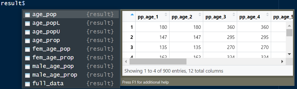Alt text Figure 2: A screenshot of result output from ‘cheesecake’ function (same as ‘cheesepop’) showing the various data frames derived from the posterior estimates. age_pop - dataframe containing predicted age groups population counts; age_popL - dataframe containing the lower bound of the predicted age groups population counts at 95% credible intervals; age_popU - dataframe containing upper bound of the predicted age groups population counts at 95% credible intervals; age_prop - dataframe containing predicted age groups population proportions; fem_age_pop - dataframe containing predicted age groups population counts for females; fem_age_prop - dataframe containing predicted age groups population proportions for females; male_age_pop - dataframe containing predicted age groups population counts for males; male_age_prop - dataframe containing predicted age groups population proportions for males.

# ... progress in R
[1] "(1) age_1 model is running"
[1] "(2) age_2 model is running"
[1] "(3) age_3 model is running"
[1] "(4) age_4 model is running"
[1] "(5) age_5 model is running"
[1] "(6) age_6 model is running"
[1] "(7) age_7 model is running"
[1] "(8) age_8 model is running"
[1] "(9) age_9 model is running"
[1] "(10) age_10 model is running"
[1] "(11) age_11 model is running"
[1] "(12) age_12 model is running"
       MAE       MAPE     RMSE    corr # model fit metrics
[1,] 3.068889 0.01599678 5.73314    1

names(result$full_data) # view column names
  [1] "admin_id"    "x1"          "x2"          "x3"          "bld"         "total"       "age_1"       "age_2"       "age_3"       "age_4"       "age_5"      
 [12] "age_6"       "age_7"       "age_8"       "age_9"       "age_10"      "age_11"      "age_12"      "total2"      "fage_1"      "fage_2"      "fage_3"     
 [23] "fage_4"      "fage_5"      "fage_6"      "fage_7"      "fage_8"      "fage_9"      "fage_10"     "fage_11"     "fage_12"     "mage_1"      "mage_2"     
 [34] "mage_3"      "mage_4"      "mage_5"      "mage_6"      "mage_7"      "mage_8"      "mage_9"      "mage_10"     "mage_11"     "mage_12"     "lon"        
 [45] "lat"         "pp_age_1"    "pp_age_2"    "pp_age_3"    "pp_age_4"    "pp_age_5"    "pp_age_6"    "pp_age_7"    "pp_age_8"    "pp_age_9"    "pp_age_10"  
 [56] "pp_age_11"   "pp_age_12"   "pp_age_1L"   "pp_age_2L"   "pp_age_3L"   "pp_age_4L"   "pp_age_5L"   "pp_age_6L"   "pp_age_7L"   "pp_age_8L"   "pp_age_9L"  
 [67] "pp_age_10L"  "pp_age_11L"  "pp_age_12L"  "pp_age_1U"   "pp_age_2U"   "pp_age_3U"   "pp_age_4U"   "pp_age_5U"   "pp_age_6U"   "pp_age_7U"   "pp_age_8U"  
 [78] "pp_age_9U"   "pp_age_10U"  "pp_age_11U"  "pp_age_12U"  "prp_age_1"   "prp_age_2"   "prp_age_3"   "prp_age_4"   "prp_age_5"   "prp_age_6"   "prp_age_7"  
 [89] "prp_age_8"   "prp_age_9"   "prp_age_10"  "prp_age_11"  "prp_age_12"  "prp_age_1L"  "prp_age_2L"  "prp_age_3L"  "prp_age_4L"  "prp_age_5L"  "prp_age_6L" 
[100] "prp_age_7L"  "prp_age_8L"  "prp_age_9L"  "prp_age_10L" "prp_age_11L" "prp_age_12L" "prp_age_1U"  "prp_age_2U"  "prp_age_3U"  "prp_age_4U"  "prp_age_5U" 
[111] "prp_age_6U"  "prp_age_7U"  "prp_age_8U"  "prp_age_9U"  "prp_age_10U" "prp_age_11U" "prp_age_12U" "pp_fage_1"   "pp_fage_2"   "pp_fage_3"   "pp_fage_4"  
[122] "pp_fage_5"   "pp_fage_6"   "pp_fage_7"   "pp_fage_8"   "pp_fage_9"   "pp_fage_10"  "pp_fage_11"  "pp_fage_12"  "pp_fage_1L"  "pp_fage_2L"  "pp_fage_3L" 
[133] "pp_fage_4L"  "pp_fage_5L"  "pp_fage_6L"  "pp_fage_7L"  "pp_fage_8L"  "pp_fage_9L"  "pp_fage_10L" "pp_fage_11L" "pp_fage_12L" "pp_fage_1U"  "pp_fage_2U" 
[144] "pp_fage_3U"  "pp_fage_4U"  "pp_fage_5U"  "pp_fage_6U"  "pp_fage_7U"  "pp_fage_8U"  "pp_fage_9U"  "pp_fage_10U" "pp_fage_11U" "pp_fage_12U" "prp_fage_1" 
[155] "prp_fage_2"  "prp_fage_3"  "prp_fage_4"  "prp_fage_5"  "prp_fage_6"  "prp_fage_7"  "prp_fage_8"  "prp_fage_9"  "prp_fage_10" "prp_fage_11" "prp_fage_12"
[166] "prp_mage_1"  "prp_mage_2"  "prp_mage_3"  "prp_mage_4"  "prp_mage_5"  "prp_mage_6"  "prp_mage_7"  "prp_mage_8"  "prp_mage_9"  "prp_mage_10" "prp_mage_11"
[177] "prp_mage_12" "pp_mage_1"   "pp_mage_2"   "pp_mage_3"   "pp_mage_4"   "pp_mage_5"   "pp_mage_6"   "pp_mage_7"   "pp_mage_8"   "pp_mage_9"   "pp_mage_10" 
[188] "pp_mage_11"  "pp_mage_12"  "pp_mage_1L"  "pp_mage_2L"  "pp_mage_3L"  "pp_mage_4L"  "pp_mage_5L"  "pp_mage_6L"  "pp_mage_7L"  "pp_mage_8L"  "pp_mage_9L" 
[199] "pp_mage_10L" "pp_mage_11L" "pp_mage_12L" "pp_mage_1U"  "pp_mage_2U"  "pp_mage_3U"  "pp_mage_4U"  "pp_mage_5U"  "pp_mage_6U"  "pp_mage_7U"  "pp_mage_8U" 
[210] "pp_mage_9U"  "pp_mage_10U" "pp_mage_11U" "pp_mage_12U"

‘cheesepop’

Description

Similar to the ‘cheesecake’ function, ‘cheesepop’ disaggregates small area population estimates by age, sex, and other socio-demographic and socio-economic characteristics (e.g., ethnicity, religion, educational level, immigration status, etc), at the administrative unit level. However, unlike the ‘cheesecake’ function which uses geospatial covariates to predict missing data values, the ‘cheesepop’ does not require the use of geospatial covariates. It uses Bayesian statistical models to predict population proportions and population totals for the demographic groups of interest. Primarily designed to help users in filling population data gaps across demographic groups due to outdated or incomplete census data.

Usage

cheesepop(df, output_dir)

Arguments

df	
A data frame object containing sample data (often partially observed) on age and sex groups population data as well as the estimated overall total counts per administrative unit.

output_dir	
This is the directory with the name of the output folder where the disaggregated population proportions and population totals are automatically saved.

Value

Example

data(toydata)
result <- cheesepop(df = toydata$admin, output_dir = tempdir())

‘pyramid’

Description

This function creates population pyramid for age and sex output data from the ‘cheesecake’ or ‘cheesepop’ functions outputs. It could also be used to visualize observed age-sex compositions.

Usage

pyramid(female_pop, male_pop)

Arguments

female_pop	
A data frame containing the disaggregated population estimates for females across all ages groups. considered.

male_pop	
A data frame containing the disaggregated population estimates for males across all ages groups. considered.

Value

A graphic image of age-sex population distribution pyramid

Example

data(toydata)
result <- cheesecake(df = toydata$admin, output_dir = tempdir())
pyramid(result$fem_age_pop,result$male_age_pop)

Making pyramid graph of the observed age-sex data

female_pop <- data.frame(toydata$admin %>% dplyr::select(starts_with("fage_"))) # extract females age data
names(female_pop) <- paste0("pp_", names(female_pop)) # rename the variables by adding "pp_" as suffix to the existing names

male_pop <- data.frame(toydata$admin %>% dplyr::select(starts_with("mage_")))# extract males age data
names(male_pop) <- paste0("pp_", names(male_pop))# rename the variables by adding "pp_" as suffix to the existing names

pyramid(female_pop,male_pop) # make the observed pyramid plot

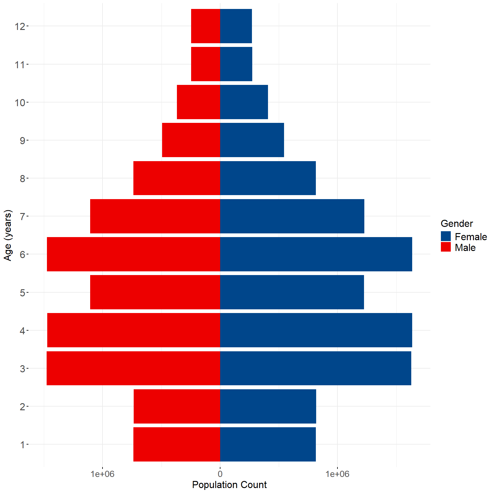Alt text Figure 3: Example of pyramid graph from ‘cheesecake’, ‘cheesepop’, ‘sprinkle’, ‘splash’ or ‘spray’ functions which produce two-level disaggregations (e.g., age and sex).

‘spices’

Description

Disaggregates population counts for a single level of demographics (e.g., age groups only or sex group only) with covariates.

Usage

spices(df, output_dir, class)

Arguments

df	
A data frame object containing sample data (often partially observed) on age or sex groups population data as well as the estimated overall total counts per administrative unit.

output_dir	
This is the directory with the name of the output folder where the disaggregated population proportions and population totals are automatically saved.

class	
This a vector which provides the levels of the categorical demographic characteristics of interest. For example, for disaggregating population by educational level, class could be the vector containing the elements "no education", "primary education", "secondary education", "tertiary education", etc.

Value

A list of data frame objects of the output files including the disaggregated population proportions and population totals along with the corresponding measures of uncertainties (lower and upper bounds of 95-percent credible intervals) for each demographic characteristic. In addition, a file containing the model performance/model fit evaluation metrics is also produced.

Example

data(toydata)
library(dplyr)
classes <- names(toydata$admin %>% dplyr::select(starts_with("age_")))
result2 <- spices(df = toydata$admin, output_dir = tempdir(), class = classes)

‘slices’

Description

This function disaggregates population estimates by a single demographic (age or sex or religion, etc) - with no geospatial covariates. Please use spices if covariates are required.

Usage

slices(df, output_dir, class)

Arguments

df	
A data frame object containing sample data (often partially observed) on age or sex groups population data as well as the estimated overall total counts per administrative unit.

output_dir	
This is the directory with the name of the output folder where the disaggregated population proportions and population totals are automatically saved.

class	
This a vector which provides the levels of the categorical demographic characteristics of interest. For example, for disaggregating population by educational level, class could be the vector containing the elements "no education", "primary education", "secondary education", "tertiary education", etc.

Value

Example

data(toydata)
library(dplyr)
classes <- names(toydata$admin %>% dplyr::select(starts_with("age_")))
result2 <- slices(df = toydata$admin, output_dir = tempdir(), class = classes)

‘sprinkle’

Description

Disaggregates population counts at high-resolution grid cells using the grid cell’s total population counts. Note that this could also be applied to more than two levels scenarios.

Usage

sprinkle(df, rdf, rclass, output_dir)

Arguments

df	
A data frame object containing sample data (often partially observed) on different demographic groups population. It contains the admin's total populatioin count to be disaggregated as well as other key variables as defined within the 'toydata'.

rdf
A gridded data frame object containing key information on the grid cells. Variables include the admin_id which must be identical to the one in the admin level data. It contains GPS coordinates. i.e, longitude (lon) and Latitude (lat) of the grid cell's centroids.

rclass	
This is a user-defined names of the files to be saved in the output folder.

output_dir	
This is the directory with the name of the output folder where the disaggregated population proportions and population totals are automatically saved.

Value

Example

# load necessary libraries
library(raster)
library(terra)
# load toy data
data(toydata)
# run 'cheesepop' function for admin level disaggregation
result <- cheesepop(df = toydata$admin,output_dir = tempdir())

rclass <- paste0("TOY_population_v1_0_age",1:12) # names of the raster files as saved in the output folder.

> rclass
 [1] "TOY_population_v1_0_age1"  "TOY_population_v1_0_age2"  "TOY_population_v1_0_age3"  "TOY_population_v1_0_age4" 
 [5] "TOY_population_v1_0_age5"  "TOY_population_v1_0_age6"  "TOY_population_v1_0_age7"  "TOY_population_v1_0_age8" 
 [9] "TOY_population_v1_0_age9"  "TOY_population_v1_0_age10" "TOY_population_v1_0_age11" "TOY_population_v1_0_age12"

# run 'sprinkle' function for grid cell disaggregation and save
result2 <- sprinkle(df = result$full_data, rdf = toydata$grid, rclass, output_dir = tempdir())

> names(result2$full_data) # view columns of the output full data.
  [1] "admin_id"    "grd_id"      "total"       "bld"         "lon"         "lat"         "pp_age_1"    "pp_age_2"    "pp_age_3"   
 [10] "pp_age_4"    "pp_age_5"    "pp_age_6"    "pp_age_7"    "pp_age_8"    "pp_age_9"    "pp_age_10"   "pp_age_11"   "pp_age_12"  
 [19] "pp_age_1L"   "pp_age_2L"   "pp_age_3L"   "pp_age_4L"   "pp_age_5L"   "pp_age_6L"   "pp_age_7L"   "pp_age_8L"   "pp_age_9L"  
 [28] "pp_age_10L"  "pp_age_11L"  "pp_age_12L"  "pp_age_1U"   "pp_age_2U"   "pp_age_3U"   "pp_age_4U"   "pp_age_5U"   "pp_age_6U"  
 [37] "pp_age_7U"   "pp_age_8U"   "pp_age_9U"   "pp_age_10U"  "pp_age_11U"  "pp_age_12U"  "prp_age_1"   "prp_age_2"   "prp_age_3"  
 [46] "prp_age_4"   "prp_age_5"   "prp_age_6"   "prp_age_7"   "prp_age_8"   "prp_age_9"   "prp_age_10"  "prp_age_11"  "prp_age_12" 
 [55] "prp_age_1L"  "prp_age_2L"  "prp_age_3L"  "prp_age_4L"  "prp_age_5L"  "prp_age_6L"  "prp_age_7L"  "prp_age_8L"  "prp_age_9L" 
 [64] "prp_age_10L" "prp_age_11L" "prp_age_12L" "prp_age_1U"  "prp_age_2U"  "prp_age_3U"  "prp_age_4U"  "prp_age_5U"  "prp_age_6U" 
 [73] "prp_age_7U"  "prp_age_8U"  "prp_age_9U"  "prp_age_10U" "prp_age_11U" "prp_age_12U" "pp_fage_1"   "pp_fage_2"   "pp_fage_3"  
 [82] "pp_fage_4"   "pp_fage_5"   "pp_fage_6"   "pp_fage_7"   "pp_fage_8"   "pp_fage_9"   "pp_fage_10"  "pp_fage_11"  "pp_fage_12" 
 [91] "pp_fage_1L"  "pp_fage_2L"  "pp_fage_3L"  "pp_fage_4L"  "pp_fage_5L"  "pp_fage_6L"  "pp_fage_7L"  "pp_fage_8L"  "pp_fage_9L" 
[100] "pp_fage_10L" "pp_fage_11L" "pp_fage_12L" "pp_fage_1U"  "pp_fage_2U"  "pp_fage_3U"  "pp_fage_4U"  "pp_fage_5U"  "pp_fage_6U" 
[109] "pp_fage_7U"  "pp_fage_8U"  "pp_fage_9U"  "pp_fage_10U" "pp_fage_11U" "pp_fage_12U" "pp_mage_1"   "pp_mage_2"   "pp_mage_3"  
[118] "pp_mage_4"   "pp_mage_5"   "pp_mage_6"   "pp_mage_7"   "pp_mage_8"   "pp_mage_9"   "pp_mage_10"  "pp_mage_11"  "pp_mage_12" 
[127] "pp_mage_1L"  "pp_mage_2L"  "pp_mage_3L"  "pp_mage_4L"  "pp_mage_5L"  "pp_mage_6L"  "pp_mage_7L"  "pp_mage_8L"  "pp_mage_9L" 
[136] "pp_mage_10L" "pp_mage_11L" "pp_mage_12L" "pp_mage_1U"  "pp_mage_2U"  "pp_mage_3U"  "pp_mage_4U"  "pp_mage_5U"  "pp_mage_6U" 
[145] "pp_mage_7U"  "pp_mage_8U"  "pp_mage_9U"  "pp_mage_10U" "pp_mage_11U" "pp_mage_12U"

ras2<- rast(paste0(output_dir = tempdir(), "/pop_TOY_population_v1_0_age4.tif")) # read in one of the saved rasters for checks, if required. 

> ras2 # view properties of the raster file
class       : SpatRaster 
dimensions  : 120, 120, 1  (nrow, ncol, nlyr)
resolution  : 0.0083, 0.0083  (x, y)
extent      : 0.00000000000000001301043, 0.996, 0.004, 1  (xmin, xmax, ymin, ymax)
coord. ref. : lon/lat WGS 84 (CRS84) (OGC:CRS84) 
source      : pop_TOY_population_v1_0_age4.tif 
name        : pop_TOY_population_v1_0_age4 
min value   :                         1.73 
max value   :                      4429.04

plot(ras2) # visualize raster

‘sprinkle1’

Description

Disaggregates population counts at high-resolution grid cells using the grid’s total population for a single level of demographics (e.g., age or sex).

Usage

sprinkle1(df, rdf, class, rclass, output_dir)

Arguments

df	
A data frame object containing sample data (often partially observed) on different demographic groups population. It contains the admin's total populatioin count to be disaggregated as well as other key variables as defined within the 'toydata'.

rdf	
A gridded data frame object containing key information on the grid cells. Variables include the admin_id which must be identical to the one in the admin level data. It contains GPS coordinates. i.e, longitude (lon) and Latitude (lat) of the grid cell's centroids.

class	
These are the categories of the variables of interest. For example, for educational level, it could be 'no education', ' primary education', 'secondary education', 'tertiary education'.

rclass	
This is a user-defined names of the files to be saved in the output folder.

output_dir	
This is the directory with the name of the output folder where the disaggregated population proportions and population totals are automatically saved.

Value

Example

 # load relevant libraries
library(raster)
library(dplyr)
library(terra)
# load the toy data
data(toydata)
 # run 'cheesepop' function for admin level disaggregation
result <- cheesepop(df = toydata$admin,output_dir = tempdir())
class <- names(toydata$admin %>% dplyr::select(starts_with("age_")))

rclass <- paste0("TOY_population_v1_0_age",1:12)
  # run 'sprinkle1' function for grid cell disaggregation at one level
result2 <- sprinkle1(df = result$full_data,
rdf = toydata$grid, class, rclass, output_dir = tempdir())
ras2<- rast(paste0(output_dir = tempdir(), "/pop_TOY_population_v1_0_age4.tif"))
plot(ras2) # visulize raster

‘splash’

Description

Disaggregates population counts at high-resolution grid cells using building counts values of grid cells as a weighting layer. It is used for two-level disaggregation (e.g., age and sex).It first disaggregates the admin unit’s total population across the grid cells. Then, each grid cell’s total count is further disaggregated into groups of interest using the admin’s proportions.

Usage

splash(df, rdf, rclass, output_dir)

Arguments

df	
A data frame object containing sample data (often partially observed) on different demographic groups population. It contains the admin's total population count to be disaggregated as well as other key variables as defined within the 'toydata'.

rdf	
A gridded data frame object containing key information on the grid cells. Variables include the admin_id which must be identical to the one in the admin level data. It contains GPS coordinates. i.e, longitude (lon) and Latitude (lat) of the grid cell's centroids.

rclass	
This is a user-defined names of the files to be saved in the output folder.

output_dir	
This is the directory with the name of the output folder where the disaggregated population proportions and population totals are automatically saved.

Value

Example

# load key libraries
# load key libraries
library(raster)
library(dplyr)
library(terra)
 # load toy data
data(toydata)
 # run 'cheesepop' to obtain admin-level proportions
result <- cheesepop(df = toydata$admin,output_dir = tempdir())
 # specify the names to assign to the raster files
rclass <- paste0("TOY_population_v1_0_age",1:12)
  # run the splash function to disaggregate at grid cells
result2 <- splash(df = result$full_data, rdf = toydata$grid, rclass, output_dir = tempdir())
  # read and visualise one of the saved raster files
ras2<- rast(paste0(output_dir = tempdir(), "/pop_TOY_population_v1_0_age4.tif"))
plot(ras2)

‘splash1’

Description

Disaggregates population counts at high-resolution grid cells using building counts values of grid cells as a weighting layer. However, unlike ‘splash’ it is used for one-level disaggregation.

Usage

splash1(df, rdf, class, rclass, output_dir)

Arguments

df	
A data frame object containing sample data (often partially observed) on different demographic groups population. It contains the admin's total populatioin count to be disaggregated as well as other key variables as defined within the 'toydata'.

rdf	
A gridded data frame object containing key information on the grid cells. Variables include the admin_id which must be identical to the one in the admin level data. It contains GPS coordinates. i.e, longitude (lon) and Latitude (lat) of the grid cell's centroids.

class	
These are the categories of the variables of interest. For example, for educational level, it could be 'no education', 'primary education', 'secondary education', 'tertiary education'.

rclass	
This is a user-defined names of the files to be saved in the output folder.

output_dir	
This is the directory with the name of the output folder where the disaggregated population proportions and population totals are automatically saved.

Value

Example

# load key libraries
library(raster)
library(dplyr)
library(terra)
 # load toy data
data(toydata)
 # run 'cheesepop' to obtain admin-level proportions
result <- cheesepop(df = toydata$admin,output_dir = tempdir())
 # specify the names to assign to the raster files
 class <- names(toydata$admin %>% dplyr::select(starts_with("age_")))
rclass <- paste0("TOY_population_v1_0_age",1:12)
  # run the splash1 function to disaggregate at grid cells
result2 <- splash1(df = result$full_data, rdf = toydata$grid,
class, rclass, output_dir = tempdir())
  # read and visualise one of the saved raster files
ras2<- rast(paste0(output_dir = tempdir(), "/pop_TOY_population_v1_0_age4.tif"))
plot(ras2)

‘spray’

Description

Disaggregates population counts by dividing the admin total by the number of grid cells within the administrative units. Then admin proportions are used to further disaggregate the grid cell totals by groups. It assigns equal weights across all the grid cells within each administrative unit of interest.

Usage

spray(df, rdf, rclass, output_dir)

Arguments

df	
A data frame object containing sample data (often partially observed) on different demographic groups population. It contains the admin's total populatioin count to be disaggregated as well as other key variables as defined within the 'toydata'.

rdf	
A gridded data frame object containing key information on the grid cells. Variables include the admin_id which must be identical to the one in the admin level data. It contains GPS coordinates. i.e, longitude (lon) and Latitude (lat) of the grid cell's centroids.

rclass	
This is a user-defined names of the files to be saved in the output folder.

output_dir	
This is the directory with the name of the output folder where the disaggregated population proportions and population totals are automatically saved.

Value

Example

 # load relevant libraries
library(raster)
library(terra)
  # load toy data
data(toydata)
 # run 'cheesepop' function for admin level disaggregation
result <- cheesepop(df = toydata$admin,output_dir = tempdir())
rclass <- paste0("TOY_population_v1_0_age",1:12) # Mean
  # run 'spray' for grid cell level disaggregation
result2 <- spray(df = result$full_data, rdf = toydata$grid, rclass, output_dir = tempdir())
ras2<- rast(paste0(output_dir = tempdir(), "/pop_TOY_population_v1_0_age4.tif"))
plot(ras2) # visualize

‘spray1’

Description

This function disaggregates population estimates at grid cell levels using the building counts of each grid cell to first disaggregate the admin unit’s total population across the grid cells. Then, each grid cell’s total count is further disaggregated into groups of interest using the admin’s proportions.Disaggregates population counts at high-resolution grid cells in the absence population and building counts - for one group level only.

Usage

spray1(df, rdf, class, rclass, output_dir)

Arguments

df	
A data frame object containing sample data (often partially observed) on different demographic groups population. It contains the admin's total populatioin count to be disaggregated as well as other key variables as defined within the 'toydata'.

rdf	

df	
A data frame object containing sample data (often partially observed) on different demographic groups population. It contains the admin's total populatioin count to be disaggregated as well as other key variables as defined within the 'toydata'.

rdf	
A gridded data frame object containing key information on the grid cells. Variables include the admin_id which must be identical to the one in the admin level data. It contains GPS coordinates. i.e, longitude (lon) and Latitude (lat) of the grid cell's centroids.

class	
These are the categories of the variables of interest. For example, for educational level, it could be 'no education', 'primary education', 'secondary education', 'tertiary education'.

rclass	
This is a user-defined names of the files to be saved in the output folder.

output_dir	
This is the directory with the name of the output folder where the disaggregated population proportions and population totals are automatically saved.

Value

Example

library(raster) # load relevant libraries
library(dplyr)
library(terra)
data(toydata) # load toy data

 # run 'cheesepop' admin unit disaggregation function
result <- cheesepop(df = toydata$admin,output_dir = tempdir())
class <- class <- names(toydata$admin %>% dplyr::select(starts_with("age_")))
rclass <- paste0("TOY_population_v1_0_age",1:12)

# run spray1 grid cell disaggregation function
result2 <- spray1(df = result$full_data, rdf = toydata$grid, class, rclass, output_dir = tempdir())
ras2<- rast(paste0(output_dir = tempdir(), "/pop_TOY_population_v1_0_age4.tif"))
plot(ras2) # visulize of the raster files produced

‘boxLine’

Description

This function automatically generates two graphs that are combined together - (a) a boxplot of the distribution of the various groups’ disaggregated population counts, and (b) a line graph of the aggregated counts across all groups (e.g., total number of individuals for each group). Here, the input data could come from any of the disaggregation functions within the ‘jollofR’ package such as ‘cheesecake’, ‘cheesepop’, ‘slices’ & ‘spices’.

Usage

boxLine(dmat, xlab, ylab)

Arguments

dmat	
A data frame containing the group-structured disaggregated population estimates which could be observed or from modelled estimates based on any of the functions - cheesecake', 'cheesepop', 'slices','spices', 'spray' , 'sprinkle', 'splash', 'spray', 'sprinkle1', 'splash1', or 'spray1'. considered.

xlab	
A user-defined label for the x-axis (e.g., 'Age group').

ylab	
A user-defined label for the y-axis (e.g., 'Population count').

Value

A graphic image of two combined graphs - a boxplot and a line plot showing the distribution of the disaggregated population counts across the groups.

Example

library(ggplot2)
data(toydata)
result <- cheesepop(df = toydata$admin,output_dir = tempdir())
boxLine(dmat=result$male_age_pop,
       xlab="Age group (years)",
       ylab = "Population Count")

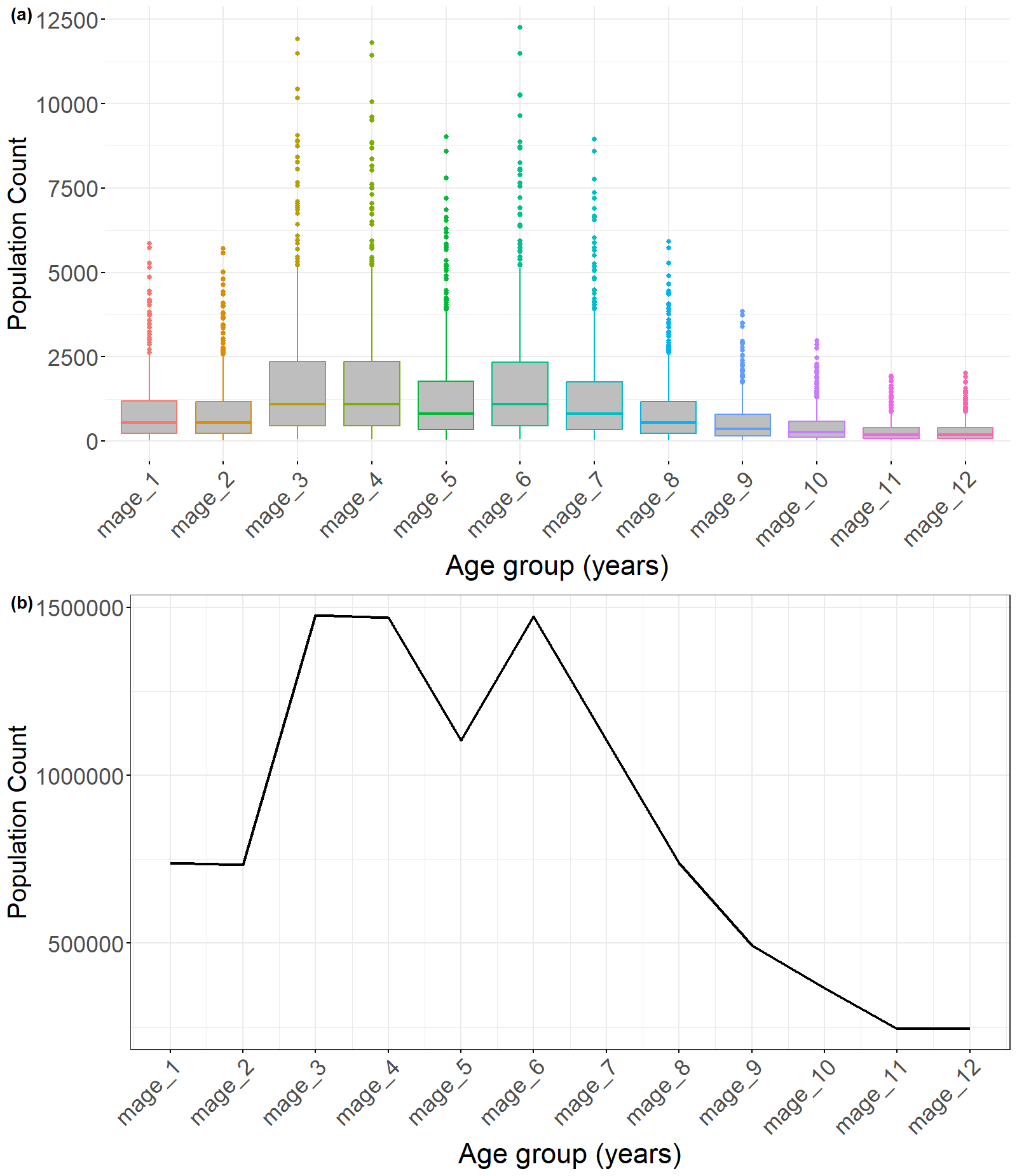Alt text Figure 4: a) Boxplots of the porterior distribution of population counts across the various age groups, and b) line plot of the aggregated population counts across all administrative units for each age group. The ‘boxLine’ function can be used for the outputs from all the jollofR disaggregation functions.

‘plotHist’

Description

This function produces a multi-panel histogram plot of the disaggregated population counts across all the groups. The input data could come from any of the disaggregation functions within the ‘jollofR’ package (both at admin and grid levels) such as ‘cheesecake’, ‘cheesepop’, ‘slices’, etc.

Usage

plotHist(dmat, xlab, ylab)

Arguments

dmat	
A data frame containing the group-structured disaggregated population estimates which could either be observed or predicted from 'cheesecake', 'cheesepop', 'slices','spices', 'spray' , 'sprinkle', 'splash', 'spray', 'sprinkle1', 'splash1', and 'spray1'.

xlab	
A user-defined label for the x-axis (e.g., 'Population Count') considered.

ylab	
A user-defined label for the y-axis (e.g., 'Frequency') considered.

Value

A graphic image of histogram of the disaggregated population count

Example

data(toydata)
library(ggplot2)
result <- cheesepop(df = toydata$admin,output_dir = tempdir())
plotHist(dmat=result$age_pop,
        xlab="Population Count",
        ylab = "Frequency")

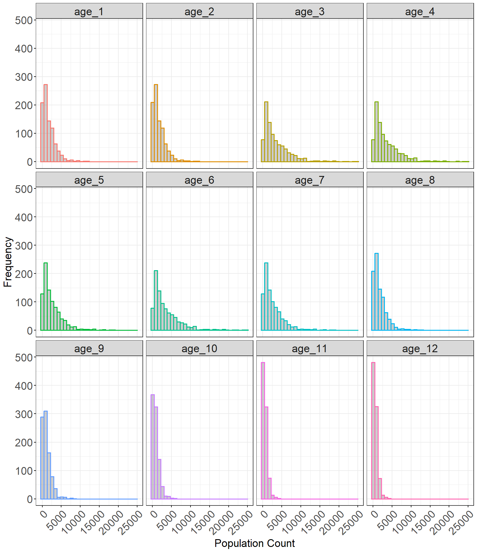Alt text Figure 5: Histograms of the posterior distribution of population counts across different age groups. The ‘plotHist’ function can be used for the outputs from all the disaggregation functions.

‘plotRast’

Description

This function produces multi-panel maps of the raster files across the various demographic groups of interest. The input data could come from any of the jollofR disaggregation functions at grid cell levels, e.g.,’sprinkle’, ‘spray’, ‘splash’, ‘sprinkle1’, ‘spray1’, and ‘splash1’.

Usage

plotRast(title, output_dir, raster_files, names, nrow, ncol)

Arguments

title	
This is the title of the multi-panel maps of the gridded structured estimates

output_dir	
The directory for saving the raster files of the disaggregated population estimates

raster_files	
The names of the raster files to visualize. This must be the same as saved in the raster output folder

names	
A user-defined names for the plot panels labels. For example, this could be the labels of different age groups. It must be the same length as the 'raster_files'.

nrow	
Number of rows of the multi-panel maps. The value depends on the number of groups being displayed.

ncol	
Number of columns of the multi-panel maps. The value depends on the number of groups being displayed. For example, for 12 raster files the products of ncol and nrow must be at least 12.

Value

A graphic image of the multi-panel maps of population disaggregated raster files

Example

data(toydata)
result <- cheesepop(df = toydata$admin,output_dir = tempdir())
rclass <- paste0("TOY_population_v1_0_age",1:12)
result2b <- spray(df=result$full_data, rdf=toydata$grid,
                 rclass, output_dir= tempdir())

# make raster maps
        #list.files(output_dir, pattern = "\.tif$",full.names = TRUE) #-
        #use this to see the list of raster files in the directory
group <- 1:12 # customised group
rclass <- paste0("TOY_population_v1_0_age",group)
plt1 <- plotRast(title = "Age disaggregated population counts", # title of the plot
output_dir = tempdir(), # directory where the raster files are saved
raster_files = paste0(output_dir=tempdir(), "/pop_",rclass, ".tif") , # raster files to plot
names = paste0("Age ", group),  # Customised names of the plot panels (same length as rclass)
nrow = 4, ncol =3)# rows and columns of the panels of the output maps
#ggsave(paste0(out_path, "/grid_maps.tif"),plot = plt1, dpi = 300) #- save in output folder

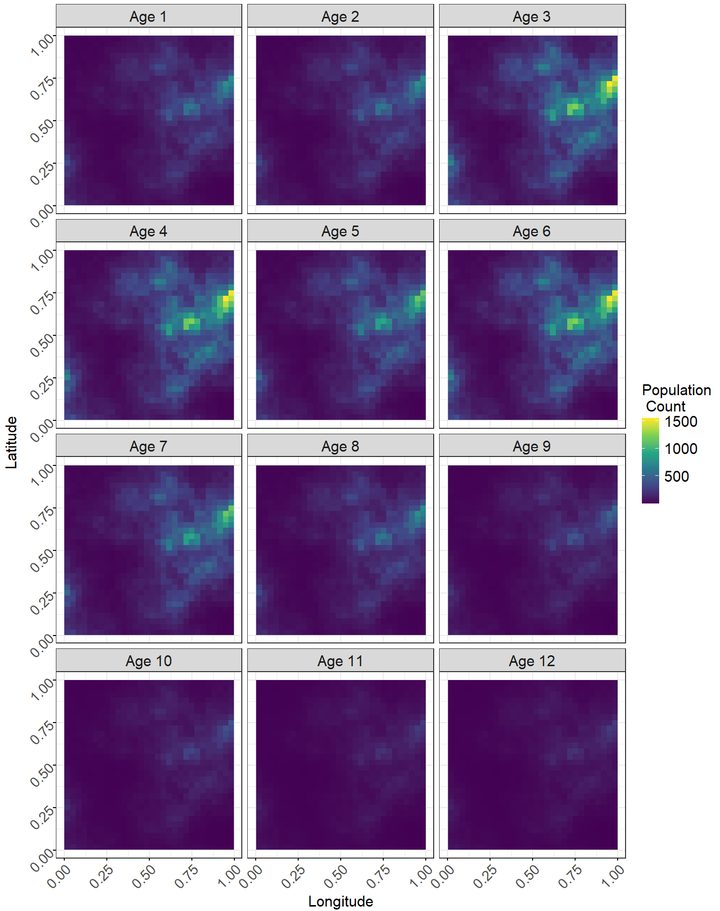Alt text Figure 6: Maps of the gridded raster files of the posterior estimates of population across the age groups. The ‘plotRast’ function can only be used to visualize outputs from the ‘sprinkle’, ‘sprinkle1’, ‘splash’, ‘splash1’, ‘spray’, and ‘spray1’ functions.

6. Model validation metrics

The jollofR package is a model-based approach which enables model validation by automatically computing model fit metrics based on the comparisons between the observed and the predicted values based on the age groups population disaggregation models. The computed metrics include:

- MAE: Mean Absolute Error
- MAPE: Mean Absolute Percentage Error
- RMSE: Root Mean Square Error
- corr: Pearson's Correlation Coefficient

7. The output files directly accessible using result$

jollofR automatically saves a number of output files as a list object. This contain 9 dataframes which can be accessed by running the function ‘result$”name_of_the_dataframe”, if the output object is called ‘result’ as in our example. These include:

age_pop: This file contains the mean disaggregated population counts by age groups. This is obtained by running the function ‘result$age_pop’
age_popL: This file contains the lower bound (2.5%) of the 95% credible interval estimates of the disaggregated population counts by age groups. This is obtained by running the function ‘result$age_popL’
age_popU: This file contains the upper bound (97.5%) of the 95% credible interval estimates of the disaggregated population counts by age groups. This is obtained by running the function ‘result$age_popU’
age_prop: This file contains the mean disaggregated population proportions by age groups. This is obtained by running the function ‘result$age_prop’
fem_age_pop: This file contains the mean disaggregated population counts by female age groups. This is obtained by running the function ‘result$fem_age_pop’
fem_age_prop: This file contains the mean disaggregated population proportions by female age groups. This is obtained by running the function ‘result$fem_age_prop’
male_age_pop: This file contains the mean disaggregated population counts by male age groups. This is obtained by running the function ‘result$male_age_pop’
male_age_prop: This file contains the mean disaggregated population proportions by male age groups. This is obtained by running the function ‘result$male_age_prop’
full_data: This file contains both the input datasets and the predicted estimates. This is obtained by running the function ‘result$full_data’

8. The output files saved in your output folder

jollofR automatically saves 8 .csv files and 1 .png file in the output folder you specified. These include:

age_disaggregated_data.csv: This file contains the mean disaggregated population counts by age groups. Variables are written as “pp_age_1, ….,pp_age_n” within the .csv file, where n is the last age group category.
age_proportions.csv: This file contains the mean disaggregated population proportions by age groups. Variables are written as “prp_age_1, ….,prp_age_n” within the .csv file, where n is the last age group category.
female_disaggregated_data.csv: This file contains the mean disaggregated population counts by female age groups. Variables are written as “pp_fage_1, ….,pp_fage_n” within the .csv file, where n is the last age group category.
female_proportions.csv: This file contains the mean disaggregated population proportions by female age groups. Variables are written as “prp_fage_1, ….,prp_fage_n” within the .csv file, where n is the last age group category.
male_disaggregated_data.csv: This file contains the mean disaggregated population counts by male age groups. Variables are written as “pp_mage_1, ….,pp_mage_n” within the .csv file, where n is the last age group category.
male_proportions.csv: This file contains the mean disaggregated population proportions by male age groups. Variables are written as “prp_mage_1, ….,prp_mage_n” within the .csv file, where n is the last age group category.
full_disaggregated_data.csv: This file contains both the input data and the posterior estimates of the disaggregated counts and proportionss.
fit_metrics.csv: This file contains the values of the model fit metrics used for model performance evaluation. Variables are written as “MAE”, “MAPE”, “RMSE”, “corr”
model_validation_scatter_plot.png: This is the automatically generated correlation plot of the observed total age data versus the model predicted total age data.

9 Statistical Modelling

The disaggregation functions within the jollofR package utilise a multi-stage hierarchical statistical modelling appraoch in which $N$ individuals within a given administrative unit (herein also called admin) of interest are assigned into only but one of the $K$ mutually exclusive and exhaustive demographic groups (e.g., age, sex, ethnicity) $group_1, group_2, …., group_K$. Then, given that $m_1, m_2, .., m_K$ are the corresponding number of individuals within the $K$ groups such that $m_j + m_{-j} = N$, where $m_j$ is the number of individuals within group j and $m_{-j}$ is the total number of individuals in the remaining $K-1$ groups ($1, 2, j-1, j+1, …,K$). Also, let $\pi_j = m_j/N$ denote the proportion of individuals belonging to group $k$, so that $\pi_{-j} = m_{-j}/N$ is the proportion of individuals not in group $j$.

We define the number of individuals belonging to group $j$ ($m_j$) as “success” while the number of individuals not belonging to group $j$ ($m_{-j}$) is the “failure” of a Binomial distribution, since the two groups are mutually exclusive and exhaustive, with a fixed number of trials (Chattamvelli & Shanmugam, 2020). Therefore, while the total number of individuals in a given administrative unit $N$ comes from a Poisson distribution with parameter $\lambda_i > 0$, the number of individuals within each group $j$ follows a Binomial distribution with mean and variance given by $N_i\pi_{ij}$ and $N_i\pi_{ij}(1-\pi_{ij})$, respectively. Then, for $i = 1, 2, … , M$, (where $M$ is the total number of administrative units of interest), the basic two-stage model is given by

\[\eqalign{ N_i \sim Poisson(\lambda_i) \\ m_{ij} \sim Binomial(N_i, \pi_{ij}) && (1) }\]

where $\lambda_i > 0$ is the mean and variance parameter of the Poisson count process for admnistrative unit $i$, and $\pi_{ij}$ is the proportion of individuals belonging to group j in admin i. Oftentimes, $N_i$ is known across all units and can be provided either through national population and housing census, Microcensus or estimated from statistical models (e.g., Leasure et al.,2020; Boo et al., 2022; Darin et al., 2022; Nnanatu et al., 2024; Nnanatu et al., 2025a; Nnanatu et al., 2025b). However, in some settings, the demographic groups-structured population counts may only be partially observed through sample surveys, for example, with missing information across some units. Here, using information within the observed group-structured data $y = (y_1, y_2, … , y_M)$, estimates of each group’s proportion can be obtained through equation (2)

\[\eqalign{ y_{ij} \sim Binomial(y_i, p_{ij}) \\ logit(p_{ij}) = X_i\beta + \xi(s) + \zeta_i \\ \zeta_i \sim Normal(0, \sigma^2_\zeta) \\ \xi(s) \sim GRF(0, \Sigma) && (2) }\]

where $y_{ij}$ is the number of individuals (partially) observed within group $j$ of admin i, such that $y_{ij} + y_{-ij} = y_i$ and $y_{-ij}$ is the total number of individuals not in group $j$. Also, $X_i$ and $\beta$ are the design matrix of geospatial covariates and the coresponding unknown fixed effects parameters, allowing us to accommodate local variabilities within the estimated group proportions. The terms $\xi(s)$ and $\zeta_i$ are the spatially varying and spatially independent random effects which account for differences due to spatial locations. In addition, the Gaussian Random Field (GRF) $\xi(s)$ allows us to more accurately estimate group-structured population counts in locations with little or no observations through shared information from nearby locations.

Finally, the predicted probability $\hat{p_{ij}} = exp(X\beta + \xi(s) + \zeta)/(1+exp(X\beta + \xi(s) + \zeta))$ provides estimates of the proportion of the individuals in group $j$ across all administrative units including those without observations, with the corresponding predicted disaggregated number $\hat{m_{ij}}$ of individuals in group $j$ of admin i given by

\[\eqalign{ \hat{m_{ij}} = \hat{p_{ij}}N_i && (3) }\]

where $N_i$ is as defined in equation (1). Note that for the above models to be valid, the proportions must add up to unity, that is, $\hat{p_{ij}} + \hat{p_{-ij}} = 1$. Parameter estimates were based on the integrated nested Laplace approximation (INLA; Rue et al., 2009), thereby enabling higher accuracy and faster computational speed. In addition, stochastic partial differential equation (SPDE; Lindgren et al., 2011) techniques were used to account for spatial autocorrelations within the sample data. However, within the jollofR version 0.3.0 package, the final model which consistently provided better fit included only the spatially independent random effect $\zeta_i$ which are implemented with covariates through the cheesecake and spices functions, or without covariates through the cheesepop and slices functions.

We illustrate the model framework example in the case of age-sex disaggregation across sex groups and 4 age groups using Figure 7 below. Here, the total population in a given administrative unit ‘total’ was first disaggregated into the 4 age agroups - ‘pp_age_1’, ‘pp_age_2’, ‘pp_age_3’, ‘pp_age_4’. Then, each age group was further disaggregated into male and female age group totals ‘pp_mage_’ and ‘pp_fage_’, respectively.

graph TD;
A[total]-->B[pp_age_1];
A[total]-->C[pp_age_2];
A[total]-->D[pp_age_3];
A[total]-->E[pp_age_4];
B[pp_age_1]-->F[pp_fage_1];
B[pp_age_1]-->G[pp_mage_1];
C[pp_age_2]-->H[pp_fage_2];
C[pp_age_2]-->I[pp_mage_2];
D[pp_age_3]-->J[pp_fage_3];
D[pp_age_3]-->K[pp_mage_3];
E[pp_age_4]-->L[pp_fage_4];
E[pp_age_4]-->M[pp_mage_4];

Figure 7: Schematic representation of age-sex disaggregation steps. Example for 4 age groups.

10 Disaggregation at high-resolution grid cells

jollofR package also allows for easy disaggregation of the estimates of population counts and proportions structured across different groups (e.g., age and sex) at high resolution grid cells. These are implemented using the ‘sprinkle’, ‘splash’ and ‘spray’ functions along with their conterparts ‘sprinkle1’, ‘splash1’ and ‘spray1’ which are used for the disaggregation of the population estimates at one group level only (e.g., age or sex). Below, we provide the descriptions of these different approaches in more details.

‘sprinkle’

The sprinkle function is used to disaggregate administrative unit i’s total population estimate $N_i$ across $K$ groups within grid cell g, based on grid cell g’s total population estimate $m_{ig}$, where $m_{ig}$ is known apriori (either from a statistical model or from other sources). That is,

\[\eqalign{ \hat{m_{ijg}} = \hat{p_{ij}}m_{ig} && (4) }\]

where $\hat{m_{ijg}}$ is the predicted number of people in group $j(j = 1,.., K)$ of grid $g$ within administrative unit $i$, and $\hat{p_{ij}}$ is the predicted proportion of group $j$ within administrative unit $i$. Note that the two key validity requirements of equation (4) here are that $\sum_jp_{ij}=1$ and $\sum_g m_{ig} = N_i$, i.e., all group proportions within admin $i$ must add up to 1, and the total population counts across all the grid cells in admin $i$ must add up to the estimated total population for admin $i$.

Note that the sprinkle1 function is also based on equation (4) under the same assumptions and validity requirements, however, as noted earlier, sprinkle1 is only used for disaggregating population for only one group level at a time. In other words, while sprinkle can be used to disaggregate into age and sex groups at the same time, for example, sprinkle1 can only be used to disaggregate either age, sex, ethnicity, educational level groups one at a time.

‘splash’

The splash function is used to disaggregate administrative unit i’s total population estimate $N_i$ across $K$ groups within grid cell g, based on grid cell g’s total building count $b_{ig}$, where $b_{ig}$ is known apriori (either from satellite imagery or other sources). That is,

\[\eqalign{ m_{ig} = w_{ig}N_i\\ \hat{m_{ijg}} = \hat{p_{ij}}m_{ig} && (5) }\]

where $m_{ig}$ is the weighted total population count of grid $g$ of admin $i$, and $w_{ig}$ is the grid $g$’s weight calculated as,

\[\eqalign{ w_{ig} = b_{ig}/\sum_g b_{ig} && (6) }\]

As before, $\hat{p_{ij}}$ is the predicted proportion of group $j$ within administrative unit $i$, and the validity requirements of equation (5) are $\sum_gw_{ig}=1$, $\sum_jp_{ij}=1$ and $\sum_g m_{ig} = N_i$. That is, all weights and group proportions within admin $i$ must add up to 1 separately, and the total population counts across all the grid cells in administrative unit $i$ must add up to the estimated total population for administrative unit $i$.

Note that the splash1 function is also based on equation (5) under the same assumptions and validity requirements, however, as noted earlier, splash1 is only used for disaggregating population for only one group level at a time. In other words, while splash can be used to disaggregate into age and sex groups at the same time, for example, splash1 can only be used to disaggregate either age, sex, ethnicity, educational level groups one at a time.

‘spray’

The spray function is used to disaggregate administrative unit i’s total population estimate $N_i$ across $K$ groups within grid cell g. The spray function is typically used when the grid cell’s total population and building counts are unknown, so that,

\[\eqalign{ m_{ig} = N_i/G_i\\ \hat{m_{ijg}} = \hat{p_{ij}}m_{ig} && (7) }\]

where $m_{ig}$ is the total population count of grid $g$ of admin unit $i$, and $G_i$ is the number of grid cells in administrative unit $i$. As before, $\hat{p_{ij}}$ is the predicted proportion of group $j$ within administrative unit $i$, and the validity requirements of equation (7) are $\sum_jp_{ij}=1$ and $\sum_g m_{ig} = N_i$. That is, all group proportions within admin unit $i$ must add up to 1, and the total population counts across all the grid cells in administrative unit $i$ must add up to the estimated total population for administrative unit $i$. Note that the spray1 function which disaggregates population counts at the grid cell level for only one group level at a time is also based on equation (7) under the same assumptions and validity requirements.

Support and Contributions

This is a development version of the jollofR package and we welcome contributions from the research community to improve jollofR and make it even much simpler for everyone to use. For support, bug reports, or feature requests, please contact:

Chris Nnanatu (Package Developer: https://www.worldpop.org/team/chris_nnanatu/)

Affiliation: Spatial Statistics & Population Modelling (SSPM) Team, WorldPop Research Group (www.worldpop.org), School of Geography and Environmental Science, University of Southampton, SO17 IBJ Southampton, United Kingdom.

Email: cc.nnanatu@soton.ac.uk or nnanatuchibuzor@gmail.com.

LinkedIn: https://www.linkedin.com/in/dr-chibuzor-christopher-nnanatu-997b68a7/

Alternatively, please feel free to open an issue on the GitHub repository via https://github.com/wpgp/jollof/issues.

Suggested citation: Nnanatu, C.C., Chaudhuri, S., Yankey, O., Lazar, A.N., Tatem, A.J.(2025). jollofR: A Bayesian statistical model-based approach for disaggregating small area population estimates by demographic characteristics. R package version 0.3.0, https://github.com/wpgp/jollofR/.

References

1) Boo, G., Darin, E., Leasure, D.R. et al.(2022). High-resolution population estimation using household survey data and building footprints. Nat Commun 13, 1330. https://doi.org/10.1038/s41467-022-29094-x 2) Chattamvelli, R., Shanmugam, R. (2020). Binomial Distribution. In: Discrete Distributions in Engineering and the Applied Sciences. Synthesis Lectures on Mathematics & Statistics. Springer, Cham. https://doi.org/10.1007/978-3-031-02425-2_2 3) Darin, E., Kuépié, M., Bassinga, H., Boo, G. & Tatem, A. J. (2022). La population vue du ciel : quand l’imagerie satellite vient au secours du recensement. Population (Wash DC). doi:10.3917/popu.2203.0467 4) Leasure, D. R., Jochem, W. C., Weber, E. M., Seaman, V. & Tatem, A. J.(2020). National population mapping from sparse survey data: A hierarchical Bayesian modeling framework to account for uncertainty. Proc Natl Acad Sci U S A 117. 5) Lindgren, F., Rue, H. & Lindström, J.(2011). An explicit link between gaussian fields and gaussian markov random fields: The stochastic partial differential equation approach. J R Stat Soc Series B Stat Methodol. doi:10.1111/j.1467-9868.2011.00777.x. 6) Nnanatu, C. et al. (2024) Modelled gridded population estimates for Cameroon 2022. Version 1.0, University of Southampton, 17 Jun 2024, DOI: 10.5258/SOTON/WP00784, https://data.worldpop.org/repo/wopr/CMR/population/v1.0/. 7) Nnanatu, C.C., et al. (2025a) Efficient Bayesian Hierarchical Small Area Population Estimation Using INLA-SPDE: Integrating Multiple Data Sources and Spatial-Autocorrelation. in Preprints; 10.20944/preprints202501.0588.v1. 8) Nnanatu, C.C., Bonnie, A., Joseph, J. et al.(2025b). Estimating small area population from health intervention campaign surveys and partially observed settlement data. Nat Commun 16, 4951. https://doi.org/10.1038/s41467-025-59862-4 9) Rue, H., Martino, S. & Chopin, N.(2009). Approximate Bayesian inference for latent Gaussian models by using integrated nested Laplace approximations. J R Stat Soc Series B Stat Methodol 71.

This site is open source. Improve this page.