Statistical population modelling for census support

class: center, middle, inverse, title-slide

# Statistical population modelling for census support
## Quiz 2
### Edith Darin

---

class: inverse, middle, center

<div>
<style type="text/css">.xaringan-extra-logo {
width: 110px;
height: 128px;
z-index: 0;
background-image: url(../../../assets/pic/320px-UNFPA_logo.svg.png);
background-size: contain;
background-repeat: no-repeat;
position: absolute;
bottom:-3.5em;left:0.5em;
}
</style>
<script>(function () {
  let tries = 0
  function addLogo () {
    if (typeof slideshow === 'undefined') {
      tries += 1
      if (tries < 10) {
        setTimeout(addLogo, 100)
      }
    } else {
      document.querySelectorAll('.remark-slide-content:not(.title-slide):not(.inverse):not(.hide_logo)')
        .forEach(function (slide) {
          const logo = document.createElement('div')
          logo.classList = 'xaringan-extra-logo'
          logo.href = null
          slide.appendChild(logo)
        })
    }
  }
  document.addEventListener('DOMContentLoaded', addLogo)
})()</script>
</div>

# Quiz

---
layout: true
# Core population model

`$$population \sim Poisson( pop\_density * settled\_area)$$`

`$$pop\_density  \sim Lognormal( \mu, \sigma)$$`
---
.center2[
In the core population model, what is `$population$`?

1. Data
2. Parameter
3. Distribution
]
---
.center2[
In the core population model, what is `$settled_area$`?

1. Data
2. Parameter
3. Distribution
]
---

.center2[
In the core population model, what is `$Lognormal$`?

1. Data
2. Parameter
3. Distribution
]

---

.center2[
In the core population model, what is `$\mu$`?

1. Data
2. Parameter
3. Distribution
]

---

.center2[
In the core population model, what is `$pop\_density$`?

1. Data
2. Parameter
3. Distribution
]

---
layout: false

# MCMC setting
A common call to `stan` looks like that:

```r
fit_model2 <- rstan::stan(file = file.path('model.stan'), 
                   data = stan_data_model,
                   iter = warmup + iter, 
                   chains = chains,
                   warmup = warmup, 
                   pars = pars,
                   seed = seed)
```

.center[
Has the `seed` an impact on the estimation process?

1.Yes<br/>
2.No

]

---
# Bayesian output

.pull-left[
#### Plot 1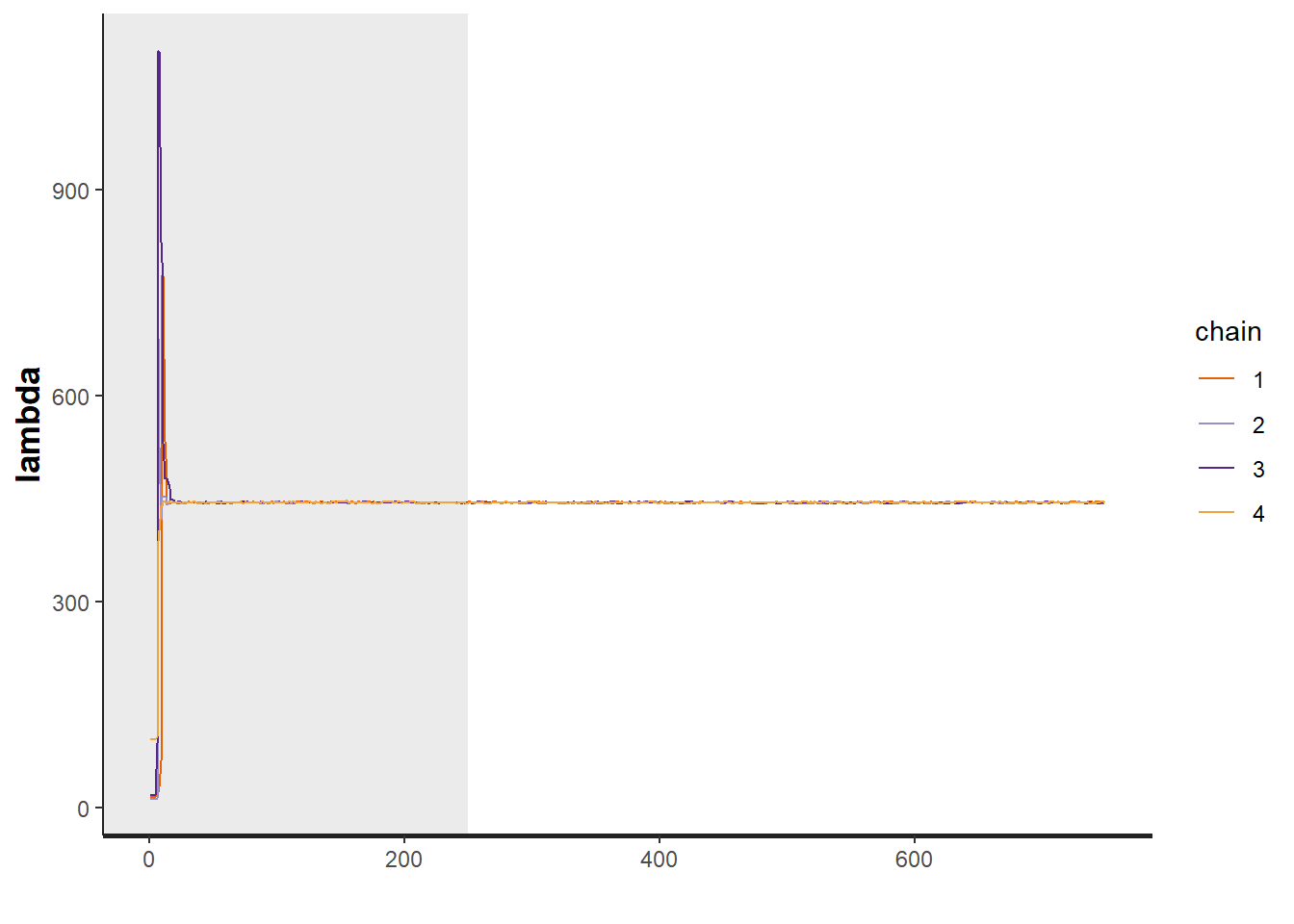
![](pic/mcq_tuto2_traceplot.png)
]
.pull-right[
#### Plot 2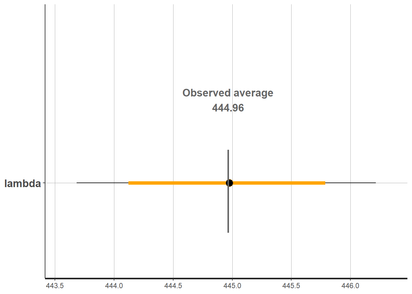
![](pic/mcq_tuto2_parameterplot.png)
]

.center[Which plot is a traceplot?

1.Plot 1<br/>
2.Plot 2
]

---
# Random modelling

.center2[*Imagine you have two groups of ten people.*

*Group A has an average height of 170 cm*<br/>
*Group B has an average height of 168 cm*

If you randomly select one person from each group who is more likely to be taller?

1. Group A
2. We don't know
]
---
layout: true
# Random modelling

.footnote[Pace~svwiki, CC BY-SA 4.0 <https://commons.wikimedia.org/w/index.php?curid=62007681>]

---
.center[
<img src="pic/mcq_tuto2_simpsonpre.PNG" alt="drawing" width="450"/>

What is the sign of the relation between x and y?

1.Positif<br/>
2.Negatif
]
---
#### Simpson's Paradox
.center[
<img src="pic/mcq_tuto2_simpsonpost.PNG" alt="drawing" width="500"/>]

---
layout: false
# Random vs hierarchical

.center2[
<img src="pic/mcq_tuto2_dag.png" alt="drawing" width="450"/>

How many models have a random effect?

1. 0
2. 1
3. 2
4. 3
]
---
layout: true
# Random vs hierarchical

`$$population \sim Poisson( pop\_density * settled\_area)$$`

`$$pop\_density \sim Lognormal( \alpha_t, \sigma)$$`

`$$\alpha_t \sim Normal( 5, 4 )$$`
---
.center2[This model represents:
1. A random model
2. A hierarchical model
]
---

.center2[This model is similar to running `$n$` models separately:
1. Yes
2. No
]

---
layout:false

# Random vs hierarchical

Gelman, Andrew. "Multilevel (hierarchical) modeling: what it can and cannot do." Technometrics 48.3 (2006): 432-435.

.center2[*Radon is a radioactive gas known to cause lung cancer in high concentrations.
Our goal is to estimate*

*(1)  the distribution of radon levels in
each of the approximately 3,000 U.S. counties and*

*(2) the impact of taking the measurement in the basement*
]
---
# Random vs hierarchical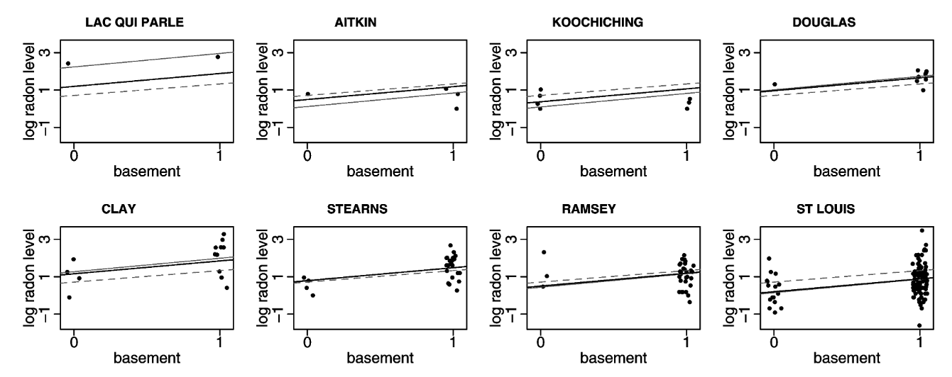

![](pic/mcq_tuto2_gelman.PNG)

.center[
The **dotted** line shows the model under:

1.No-pooling <br/>
2.Complete pooling<br/>
3.Partial pooling
]

---
# Random vs hierarchical

![](pic/mcq_tuto2_gelman.PNG)

.center[
The **light-colored** line shows the model under:

1.No-pooling <br/>
2.Complete pooling<br/>
3.Partial pooling
]

---
# Estimation in `stan`

`## Warning in validityMethod(object): The following variables have undefined values: population_hat[1],The following variables have undefined`

.center2[
Is this warning problematic
1. Yes
2. No
]

---
layout: true
# Hierarchically estimated parameters

.pull-left[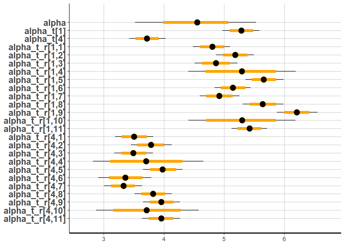![](pic/mcq_tuto2_hierarchicalalpha.png)]

---
.pull-right[What is the estimated **national** population density median (in log)?
1. 3.5
2. 4
3. 4.5
4. 5
5. 5.5
6. 6]
---

.pull-right[What is the estimated population density median for **settlement type 1** (in log)?
1. 3.5
2. 4
3. 4.5
4. 5
5. 5.5
6. 6]